Banyak orang setidaknya satu kali memiliki kebutuhan untuk menggambar peta kota atau negara dengan cepat, meletakkan datanya di sana (titik, rute, peta panas, dll.).

Cara cepat menyelesaikan masalah seperti itu, di mana mendapatkan peta kota atau negara untuk menggambar - dalam instruksi terperinci di bawah potongan.

pengantar

(, , ) .

, :

, , , , ( , / / ).

, .shp geopandas.

, :

1. —
2. "1"
3. ,

, , , .

Shapefile.

, Shapefile — , (, ), (, ).

, :

• —
• — ,
• — , \

.

OpenStreetMap ( OSM). , — , .

, . OSM.

OSM, ( , ).

NextGis, , .

NextGis ( ~30 ) — ( ~4 ). .

— , ( ) ( / ).

, , (, , , ). , , , , , .

OpenStreetMap. , .

, , , , "".

, . , , , .

, ( "").

, , , !

Geopandas, Pandas, Matplotlib Numpy.

Geopandas pip Windows , conda install geopandas .

import pandas as pd
import numpy as np
import geopandas as gpd
from matplotlib import pyplot as plt

Shapefile

zip .

data . , ( .shp) ( .cpg, .dbf, .prj, .shx).

, geopandas:

• . , 1.2GB, 22.8GB. , — ( geopandas )
• . , 'cp1251', — 'utf-8'
• , , - . .

#    data   
#       zip-     
ZIP_PATH = 'zip://C:/Users/.../Moscow.zip!data/'

#        shp 
LAYERS_DICT = {
    'boundary_L2': 'boundary-polygon-lvl2.shp', #    
    'boundary_L4': 'boundary-polygon-lvl4.shp',
    'boundary_L5': 'boundary-polygon-lvl5.shp',
    'boundary_L8': 'boundary-polygon-lvl8.shp',
    'building_point': 'building-point.shp',  # ,    
    'building_poly': 'building-polygon.shp'  # ,    
              }

#        
i = 0
for layer in LAYERS_DICT.keys():

    path_to_layer = ZIP_PATH + LAYERS_DICT[layer]

    if layer[:8]=='boundary':
        encoding = 'cp1251'
    else:
        encoding = 'utf-8'
    globals()[layer] = gpd.read_file(path_to_layer, encoding=encoding)

    i+=1
    print(f'[{i}/{len(LAYERS_DICT)}] LOADED {layer} WITH ENCODING {encoding}')

:

[1/6] LOADED boundary_L2 WITH ENCODING cp1251
[2/6] LOADED boundary_L4 WITH ENCODING cp1251
[3/6] LOADED boundary_L5 WITH ENCODING cp1251
[4/6] LOADED boundary_L8 WITH ENCODING cp1251
[5/6] LOADED building_point WITH ENCODING utf-8
[6/6] LOADED building_poly WITH ENCODING utf-8

GeoDataFrame, . :

fig, (ax1, ax2, ax3, ax4) = plt.subplots(1, 4, figsize=(15,15))
boundary_L2.plot(ax=ax1, color='white', edgecolor='black')
boundary_L4.plot(ax=ax2, color='white', edgecolor='black')
boundary_L5.plot(ax=ax3, color='white', edgecolor='black')
boundary_L8.plot(ax=ax4, color='white', edgecolor='black')

, , OSM. — .

. - , .

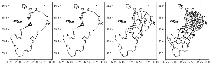
building_poly.plot(figsize=(10,10))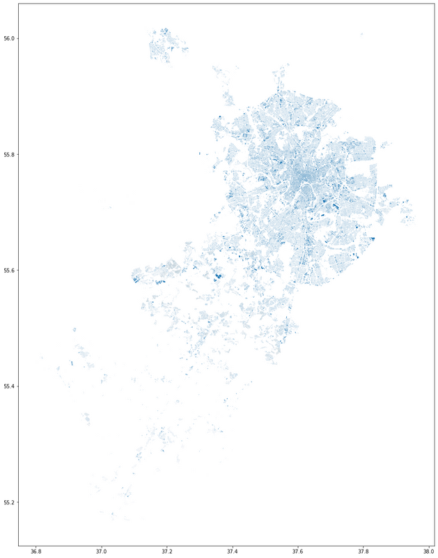

:

base = boundary_L2.plot(color='white', alpha=.8, edgecolor='black', figsize=(50,50))
boundary_L8.plot(ax=base, color='white', edgecolor='red', zorder=-1)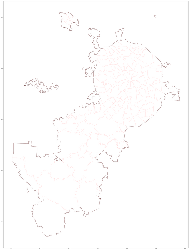

gpd.

, Geopandas Pandas. , (, ), , .

boundary_L8.head()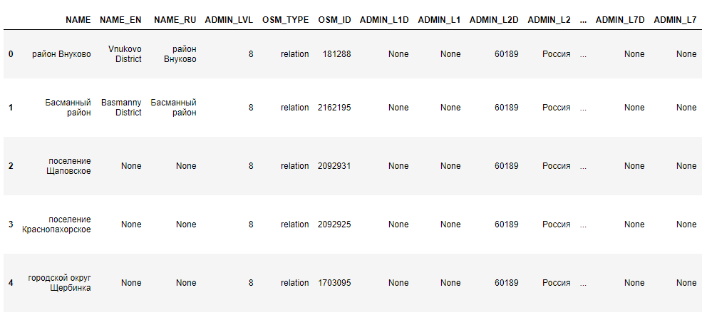

2:

• OSM_ID — OpenStreetMap
• geometry —

.

, , :

print('POLYGONS')
print('# buildings total', building_poly.shape[0])
building_poly = building_poly.loc[building_poly['A_PSTCD'].notna()]
print('# buildings with postcodes', building_poly.shape[0])
print('\nPOINTS')
print('# buildings total', building_point.shape[0])
building_point = building_point.loc[building_point['A_PSTCD'].notna()]
print('# buildings with postcodes', building_point.shape[0])

:

POLYGONS
# buildings total 241511
# buildings with postcodes 13198

POINTS
# buildings total 1253
# buildings with postcodes 4

, , ( , 5%, 13 ).

:

2. OSM-ID ,
3. , "" . , , .

%%time
building_areas = gpd.GeoDataFrame(building_poly[['A_PSTCD', 'geometry']])
building_areas['area'] = 'NF'

#     ,         

#      ,          .centroid.
#      ,      

for area in boundary_L8['OSM_ID']: 
    area_geo = boundary_L8.loc[boundary_L8['OSM_ID']==area, 'geometry'].iloc[0]
    nf_buildings = building_areas['area']=='NF' #       ,      
    building_areas.loc[nf_buildings, 'area'] = np.where(building_areas.loc[nf_buildings, 'geometry'].centroid.within(area_geo), area, 'NF')

#  ,     ,    -  .
#       ,      .
codes_pivot = pd.pivot_table(building_areas,
                             index='A_PSTCD',
                             columns='area',
                             values='geometry',
                             aggfunc=np.count_nonzero)

#  ,           
codes_pivot['main_area'] = codes_pivot.idxmax(axis=1)

#       ""   
for pst_code in codes_pivot.index:
    main_area = codes_pivot.loc[codes_pivot.index==pst_code, 'main_area']
    share = codes_pivot.loc[codes_pivot.index==pst_code, main_area].iloc[0,0] / codes_pivot.loc[codes_pivot.index==pst_code].sum(axis=1)*100
    codes_pivot.loc[codes_pivot.index==pst_code, 'share_in_main_area'] = int(share)

#     
codes_pivot = codes_pivot.loc[:, ['main_area', 'share_in_main_area']].fillna(0)

:

, , , , ( , ).

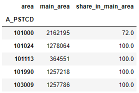
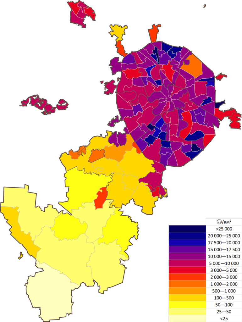
: "1".

#     - 
codes_pivot['count_1'] = codes_pivot.index.str.count('1')
#      
areas_pivot = pd.pivot_table(codes_pivot, index='main_area', values='count_1', aggfunc=np.mean)
areas_pivot.index = areas_pivot.index.astype('int64')
#        
boundary_L8_w_count = boundary_L8.merge(areas_pivot, how='left', left_on='OSM_ID', right_index=True)
#   
boundary_L8_w_count.plot(column='count_1', legend=True, figsize=(10,10))

:

, — ,

, , , .

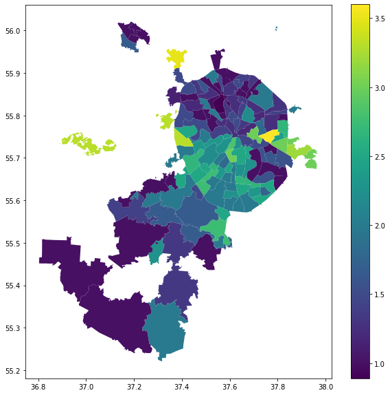
— share_in_main_area

, "" :

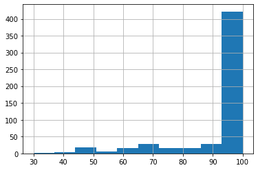
codes_pivot[codes_pivot['share_in_main_area']>50].shape[0]/codes_pivot.shape[0]

:

0.9568345323741008

.

Geopandas — . Matplotlib Pandas .

OSM — , .

, !

— .