👨‍🏫 🛋️ 😂 Aplikasi cabul 💶 ♥️ 🏭

Dalam lampiran artikel, jalur partikel menyediakan bahan potong: jalur integral, percobaan dua celah pada atom neon dingin, bingkai teleportasi partikel, dan adegan lain dari kekejaman dan sifat seksual.

Menurut pendapat saya, tidak ada cara lain untuk menganggap formalisme matematika sebagai konsisten secara logis selain menunjukkan bahwa konsekuensinya menyimpang dari pengalaman, atau untuk membuktikan bahwa ramalannya tidak menguras kemungkinan pengamatan.

Niels Bohr

Sebagai kesimpulan, penulis ingin menyatakan bahwa kita hanya mengenali dua alasan bagus untuk meninggalkan teori yang menjelaskan berbagai fenomena. Pertama, teori ini tidak konsisten secara internal, dan kedua, tidak setuju dengan eksperimen.

David Bohm

Sebelumnya kami telah belajar dari mana persamaan Schrödinger berasal, mengapa persamaan ini diambil dari sana, dan bagaimana persamaan ini diambil dengan berbagai metode

i ℏ \frac{\partial Ψ}{\partial t} = (- \frac{ℏ^{2}}{2 m} \nabla^{2} + V) Ψ

$i\hbar\frac{\partial\Psi}{\partial t} = \left( -\frac{\hbar^2}{2m}\nabla^2 + V\right) \Psi$

Sekarang, mari kita bagi menjadi dua persamaan nyata. Untuk melakukan ini, kami mewakili psi dalam bentuk kutub $\Psi = Re^{iS/\hbar}$ , :

\frac{\partial S}{\partial t} + \frac{(\nabla S)^{2}}{2 m} - \frac{ℏ^{2}}{2 m} \frac{\nabla^{2} R}{R} + V = 0 \frac{\partial R^{2}}{\partial t} + \nabla \cdot (\frac{R^{2} \nabla S}{m}) = 0

$\frac{\partial S}{\partial t}+\frac{(\nabla S)^{2}}{2 m}-\frac{\hbar^{2}}{2 m} \frac{\nabla^{2} R}{R}+V=0 \\ \frac{\partial R^{2}}{\partial t}+\nabla \cdot\left(\frac{R^{2} \nabla S}{m}\right)=0$

S — , R — . , , , — -, ( ).

, $U = \nabla S /m$ . , S -, - - :

S = - \frac{i ℏ}{2} \ln \frac{Ψ}{Ψ^{*}}

$S = -\frac{i\hbar}{2}\ln\frac{\Psi}{\Psi^*}$

, -, , , , S, , , , . , , . -.

— , . , , , . , , , .

, , , . . . , , , .

, .

, , , . , ( - ). :

()

, , , : ,

, . . .

U = \nabla S / m = - \frac{i ℏ}{2 m} \nabla \ln \frac{Ψ}{Ψ^{*}} = \frac{ℏ}{m} I m (\frac{\nabla ψ}{ψ})

$U = \nabla S /m = -\frac{i\hbar}{2m}\nabla\ln\frac{\Psi}{\Psi^*} = \frac{\hbar}{m}\mathrm{Im}\left(\frac{\nabla\psi}{\psi} \right)$

-, :

x + = U Δ t

$x += U\Delta t$

using LinearAlgebra, SparseArrays, Plots

const ħ = 1.0546e-34 # J*s
const m = 9.1094e-31 # kg
const q = 1.6022e-19 # Kl
const nm = 1e-9 # m
const fs = 1e-12; # s

function wavefun()

    gauss(x) = exp( -(x-x0)^2 / (2*σ^2) + im*x*k )
    k = m*v/ħ

    #    
    Vm = spdiagm(0 => V )
    H = spdiagm(-1 => ones(Nx-1), 0 => -2ones(Nx), 1 => ones(Nx-1) )
    H *= ħ^2 / ( 2m*dx^2 )
    H += Vm

    A = I + 0.5im*dt/ħ * H #  
    B = I - 0.5im*dt/ħ * H # 
    psi = zeros(Complex, Nx, Nt)
    psi[:,1] = gauss.(x)

    for t = 1:Nt-1

        b = B * psi[:,t]
        #       A*psi = b
        psi[:,t+1] = A \ b
    end

    return psi
end

dx = 0.05nm # x step
dt = 0.01fs # t step
xlast = 400nm
Nt = 260 # Number of time steps
t = range(0, length = Nt, step = dt)

x = [0:dx:xlast;]
Nx = length(x) # Number of spatial steps

a1 = 200nm
a2 = 200.5nm # 5 
a3 = 205nm
a4 = 205.5nm 
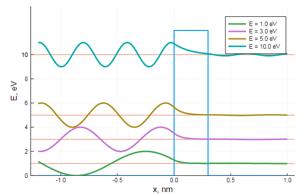
#V = [ a1<xi<a2 ? 2q : 0.0 for xi in x ] # 2 eV 
V = [ a1<xi<a2 || a3<xi<a4 ? 2q : 0.0 for xi in x ] # 2 eV 

x0 = 80nm # Initial position
σ = 20nm # gauss width
v = -120nm/fs;

@time Psi = wavefun()
P = abs2.(Psi);

function ψ(xi, j)

    k = findfirst(el-> abs(el-xi)<dx, x)
    k == nothing && ( k = 1 )

    Psi[k, j]
end

function corpusculaz(n)

    X = zeros(n, Nt)
    X[:,1] = x0 .+ σ*randn(n)

    for j in 2:Nt, i in 1:n
        U = ħ/(2m*dx) * imag( ( ψ(X[i,j-1]+dx, j) -  ψ(X[i,j-1]-dx, j) ) /  ψ(X[i,j-1], j) )
        X[i,j] = X[i,j-1] - U*dt
    end

    X
end

@time X = corpusculaz(20);

plot(x, P[:, 1], legend = false)
plot!(x, P[:, 80], legend = false)
scatter!( X[:,1], zeros(20) )
scatter!( X[:,80], zeros(20) )

. — , . :

, . , , !

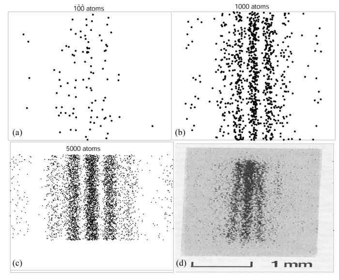
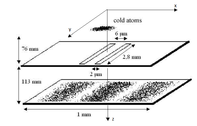
, . Double-slit interference with ultracold metastable neon atoms — - .

using Random, Gnuplot, Statistics
#  
function trapez(f, a, b, n)
    h = (b - a)/n
    result = 0.5*(f(a) + f(b))
    for i in 1:n-1
        result += f(a + i*h)
    end
    result * h
end
#  
function rk4(f, x, y, h)
    k1 = h * f(x       , y        )
    k2 = h * f(x + 0.5h, y + 0.5k1)
    k3 = h * f(x + 0.5h, y + 0.5k2)
    k4 = h * f(x +    h, y +    k3)

    return y + (k1 + 2*(k2 + k3) + k4)/6.0
end

const ħ = 1.055e-34 # J*s 
const kB = 1.381e-23 # J*K-1
const g = 9.8 # m/s^2

const l1 = 76e-3 # m
const l2 = 113e-3 # m
const yh = 2.8e-3 # m
const d = 6e-6 # m
const b = 2e-6 # m
const a1 = 0.5(- d - b) # 
const a2 = 0.5(- d + b)
const b1 = 0.5(  d - b)
const b2 = 0.5(  d + b)

const m = 3.349e-26 # kg
const T = 2.5e-3 # K
const σv = sqrt(kB*T/m) #  
const σ₀ = 10e-6 # 10 mkm #      
const σz = 3e-4 # 0.3 mm #  z
const σk = m*σv / (ħ*√3) # 2e8 m/s #    

v₀ = zeros(3)
k₀ = zeros(3);

: , , -, .

\begin{aligned} 1) ψ_{0} (x, y, z; k_{0 x}, k_{0 y}, k_{0 z}) = & ψ_{0 x} (x; k_{0 x}) ψ_{0_{y}} (z; k_{0 y}) ψ_{0 z} (z; k_{0 z}) \\ = & {(2 π σ_{0}^{2})}^{- 1 / 4} e^{- x^{2} / 4 σ_{0}^{2}} e^{i k_{0 x} x} \\ \times {(2 π σ_{0}^{2})}^{- 1 / 4} e^{- y^{2} / 4 σ_{0}^{2}} e^{i k_{0 y} y} \\ \times {(2 π σ_{z}^{2})}^{- 1 / 4} e^{- z^{2} / 4 σ_{z}^{2}} e^{i k_{0 z} z} \end{aligned}

$\begin{aligned} 1)\psi_{0}\left(x, y, z ; k_{0 x}, k_{0 y}, k_{0 z}\right)=& \psi_{0 x}\left(x ; k_{0 x}\right) \psi_{0_{y}}\left(z ; k_{0 y}\right) \psi_{0 z}\left(z ; k_{0 z}\right) \\ =&\left(2 \pi \sigma_{0}^{2}\right)^{-1 / 4} e^{-x^{2} / 4 \sigma_{0}^{2}} e^{i k_{0 x} x} \\ & \times\left(2 \pi \sigma_{0}^{2}\right)^{-1 / 4} e^{-y^{2} / 4 \sigma_{0}^{2}} e^{i k_{0 y} y} \\ & \times\left(2 \pi \sigma_{z}^{2}\right)^{-1 / 4} e^{-z^{2} / 4 \sigma_{z}^{2}} e^{i k_{0 z} z} \end{aligned}$

, . , , , . , , .

, . , , — . , , , . , , .

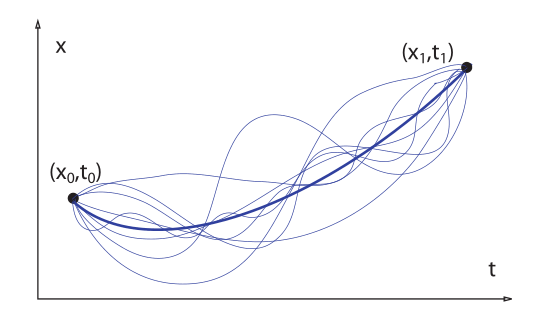
Quantum Mechanics And Path Integrals, A. R. Hibbs, R. P. Feynman, , 3.6 .

K (β, t_{β}; α, t_{α}) = K_{x} (x_{β}, t_{β}; x_{α}, t_{α}) K_{y} (y_{β}, t_{β}; y_{α}, t_{α}) K_{z} (z_{β}, t_{β}; z_{α}, t_{α})

$K\left(\beta, t_{\beta} ; \alpha, t_{\alpha}\right)=K_{x}\left(x_{\beta}, t_{\beta} ; x_{\alpha}, t_{\alpha}\right) K_{y}\left(y_{\beta}, t_{\beta} ; y_{\alpha}, t_{\alpha}\right) K_{z}\left(z_{\beta}, t_{\beta} ; z_{\alpha}, t_{\alpha}\right)$

\begin{aligned} K_{x} (x_{β}, t_{β}; x_{α}, t_{α}) = & {(\frac{m}{2 i π ℏ (t_{β} - t_{α})})}^{1 / 2} \exp \frac{i m}{ℏ} (\frac{{(x_{β} - x_{α})}^{2}}{2 (t_{β} - t_{α})}) \\ K_{y} (y_{β}, t_{β}; y_{α}, t_{α}) = & {(\frac{m}{2 i π ℏ (t_{β} - t_{α})})}^{1 / 2} \exp \frac{i m}{ℏ} (\frac{{(y_{β} - y_{α})}^{2}}{2 (t_{β} - t_{α})}) \\ K_{z} (z_{β}, t_{β}; z_{α}, t_{α}) = & {(\frac{m}{2 i π ℏ (t_{β} - t_{α})})}^{1 / 2} \exp \frac{i m}{ℏ} (\frac{{(z_{β} - z_{α})}^{2}}{2 (t_{β} - t_{α})}) \\ \times \exp \frac{i m}{ℏ} (\frac{g}{2} (z_{β} + z_{α}) (t_{β} - t_{α}) - \frac{g^{2}}{24} {(t_{β} - t_{α})}^{3}) \end{aligned}

$\begin{aligned} K_{x}\left(x_{\beta}, t_{\beta} ; x_{\alpha}, t_{\alpha}\right)=&\left(\frac{m}{2 i \pi \hbar\left(t_{\beta}-t_{\alpha}\right)}\right)^{1 / 2} \exp \frac{i m}{\hbar}\left(\frac{\left(x_{\beta}-x_{\alpha}\right)^{2}}{2\left(t_{\beta}-t_{\alpha}\right)}\right) \\ K_{y}\left(y_{\beta}, t_{\beta} ; y_{\alpha}, t_{\alpha}\right)=&\left(\frac{m}{2 i \pi \hbar\left(t_{\beta}-t_{\alpha}\right)}\right)^{1 / 2} \exp \frac{i m}{\hbar}\left(\frac{\left(y_{\beta}-y_{\alpha}\right)^{2}}{2\left(t_{\beta}-t_{\alpha}\right)}\right) \\ K_{z}\left(z_{\beta}, t_{\beta} ; z_{\alpha}, t_{\alpha}\right)=&\left(\frac{m}{2 i \pi \hbar\left(t_{\beta}-t_{\alpha}\right)}\right)^{1 / 2} \exp \frac{i m}{\hbar}\left(\frac{\left(z_{\beta}-z_{\alpha}\right)^{2}}{2\left(t_{\beta}-t_{\alpha}\right)}\right) \\ & \times \exp \frac{i m}{\hbar}\left(\frac{g}{2}\left(z_{\beta}+z_{\alpha}\right)\left(t_{\beta}-t_{\alpha}\right)-\frac{g^{2}}{24}\left(t_{\beta}-t_{\alpha}\right)^{3}\right) \end{aligned}$

Z , . ,

ψ (β, t) = \int K (β, t; α, t_{α}) ψ (α, t_{α}) d x_{α}, d y_{α}, d z_{α}

$\psi\left(\beta, t \right)=\int K\left(\beta, t ; \alpha, t_{\alpha}\right) \psi\left(\alpha, t_{\alpha}\right) d x_{\alpha}, d y_{\alpha}, d z_{\alpha}$

, . , X, . :

\begin{aligned} ψ_{x} (x, t; k_{0 x}) & = \int K (x, t; x_{α}, 0) ψ_{0} (x_{α}) d x_{α} \\ ψ_{x} (x, t; k_{0 x}) & = {(2 π s_{0}^{2} (t))}^{- 1 / 4} \exp [- \frac{{(x - v_{0 x} t)}^{2}}{4 σ_{0} s_{0} (t)} + i k_{0 x} (x - v_{0 x} t)] \\ ρ_{x} (x, t) & = {(2 π ε_{0}^{2} (t))}^{- 1 / 2} \exp [- \frac{x^{2}}{2 ε_{0}^{2} (t)}] \end{aligned}

$\begin{aligned} \psi_{x}\left(x, t ; k_{0 x}\right)&=\int K\left(x, t ; x_\alpha, 0\right) \psi_0\left(x_\alpha\right) d x_{\alpha}\\ \psi_{x}\left(x, t ; k_{0 x}\right) &=\left(2 \pi s_{0}^{2}(t)\right)^{-1 / 4} \exp \left[-\frac{\left(x-v_{0 x} t\right)^{2}}{4 \sigma_{0} s_{0}(t)}+i k_{0 x}\left(x-v_{0 x} t\right)\right] \\ \rho_{x}(x, t) &=\left(2 \pi \varepsilon_{0}^{2}(t)\right)^{-1 / 2} \exp \left[-\frac{x^{2}}{2 \varepsilon_{0}^{2}(t)}\right] \end{aligned}$

ε_{0}^{2} (t) = σ_{0}^{2} (t) + {(\frac{h t σ_{v}}{m})}^{2} σ_{0}^{2} (t) = σ_{0}^{2} + {(\frac{h t}{2 m σ_{0}^{2}})}^{2}

$\varepsilon_{0}^{2}(t)=\sigma_{0}^{2}(t)+\left(\frac{h t \sigma_v}{m}\right)^{2}\\ \sigma_{0}^{2}(t)=\sigma_{0}^{2}+\left(\frac{h t}{2 m \sigma_{0}^{2}}\right)^{2}$

, :

ε₀(t) = σ₀^2 + ( ħ/(2m*σ₀) * t )^2 + (ħ*t*σv/m)^2
s₀(t) = σ₀ + im*ħ/(2m*σ₀) * t

ρₓ(x, t) = exp( -x^2 / (2ε₀(t)) ) / sqrt( 2π*ε₀(t) )

t₁(v, z) = sqrt( 2*(l1-z)/g + (v/g)^2 ) - v/g
tf1 = t₁(v₀[3], 0) # s #    
X1 = range(-100, stop = 100, length = 100)*1e-6 
Z1 = range(0, stop = l1, length = 100)
Cron1 = range(0, stop = tf1, length = 100)

P1 = [ ρₓ(x, t) for t in Cron1, x in X1 ]
P1 /= maximum(P1); #   

@gp "set title 'Wavefun before the slits'" xlab="Z, mkm" ylab="X, mkm"
@gp :- 1000Z1 1000000X1 P1 "w image notit"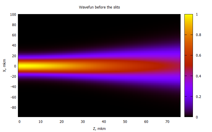

— .

, :

\begin{aligned} ψ_{x} & (x, t) = ψ_{A} + ψ_{B} \\ ψ_{A} & = \int_{A} K_{x} (x, t; x_{a}, t_{1}) ψ_{x} (x_{a}, t_{1}, k_{0 x}) d x_{a} \\ ψ_{B} & = \int_{B} K_{x} (x, t; x_{b}, t_{1}) ψ_{x} (x_{b}, t_{1}, k_{0 x}) d x_{b} \end{aligned}

$\begin{aligned} \psi_{x}&\left(x, t\right)=\psi_{A}+\psi_{B}\\ \psi_{A} &=\int_{A} K_{x}\left(x, t ; x_{a}, t_{1}\right) \psi_{x}\left(x_{a}, t_{1}, k_{0 x}\right) d x_{a} \\ \psi_{B} &=\int_{B} K_{x}\left(x, t ; x_{b}, t_{1}\right) \psi_{x}\left(x_{b}, t_{1}, k_{0 x}\right) d x_{b} \end{aligned}$

ρ_{x} (x, t) = \int_{- \infty}^{+ \infty} {(2 π σ_{v}^{2})}^{- 1 / 2} \exp (- \frac{k_{0 x}^{2}}{2 σ_{v}^{2}}) {| ψ_{x} (x, t; k_{0 x}) |}^{2} d k_{0 x}

$\rho_{x}\left(x, t\right)=\int_{-\infty}^{+\infty}\left(2 \pi \sigma_v^{2}\right)^{-1 / 2} \exp \left(-\frac{k_{0 x}^{2}}{2 \sigma_v^{2}}\right)\left|\psi_{x}\left(x, t ; k_{0 x}\right)\right|^{2} d k_{0 x}$

, :

function ρₓ(xᵢ, tᵢ) 

    Kₓ(xb, tb, xa, ta) = sqrt( m/(2im*π*ħ*(tb-ta)) ) * exp( im*m*(xb-xa)^2 / (2ħ*(tb-ta)) )

    function subintrho(k) 

        ψₓ(x, t) = ( 2π*s₀(t) )^-0.25 * exp( -(x-ħ*k*t/m)^2 / (4σ₀*s₀(t)) + im*k*(x-ħ*k*t/m) )
        subintpsi(x) = Kₓ(xᵢ, tᵢ, x, tf1) * ψₓ(x, tf1)

        ψa = trapez(subintpsi, a1, a2, 200)
        ψb = trapez(subintpsi, b1, b2, 200)

        exp( -k^2 / (2σv^2) ) * abs2(ψa + ψb)
    end

    trapez(subintrho, -10σk, 10σk, 20) / sqrt( 2π*σv^2 )
end

t₂(v, z) = sqrt( 2*(l1+l2-z)/g + (v/g)^2 ) - v/g
tf2 = t₂(v₀[3], 0) # s #    
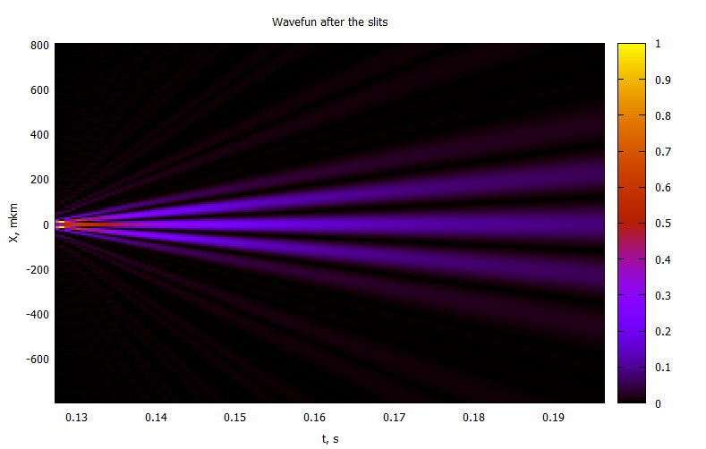
X2 = range(-800, stop = 800, length = 200)*1e-6
Z2 = range(l1, stop = l2, length = 100)
Cron2 = range(tf1, stop = tf2, length = 100)

@time P2 = [ ρₓ(x, t) for t in Cron2, x in X2 ];

P2 /= maximum(P2[4:end,:]);
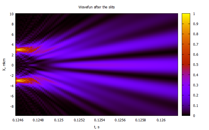
@gp "set title 'Wavefun after the slits'" xlab="t, s" ylab="X, mkm"
@gp :- Cron2[4:end] 1000000X2 P2[4:end,:] "w image notit"

2 :

\vec{v} = \frac{\nabla S}{m}

$\vec v = \frac{\nabla S}{m}$

. . , ,

\begin{aligned} \vec{v} (x, y, z, t) & = \frac{\nabla S}{m} + \frac{\nabla \log ρ \times \vec{s}}{m} \\ \vec{s} & = (0, 0, ℏ / 2) \\ \frac{\nabla \log ρ \times \vec{s}}{m} & = \frac{ℏ}{2 m ρ} (\frac{\partial ρ}{\partial y}, - \frac{\partial ρ}{\partial x}, 0) \end{aligned}

$\begin{aligned} \vec v(x, y, z, t)&=\frac{\nabla S}{m}+\frac{\nabla \log \rho \times \vec s}{m} \\ \vec s &= (0,0,\hbar/2)\\ \frac{\nabla \log \rho \times \vec s}{m} &= \frac{\hbar}{2 m \rho}\left( \frac{\partial \rho}{\partial y}, -\frac{\partial \rho}{\partial x}, 0\right) \end{aligned}$

, ,

\begin{aligned} \frac{d x}{d t} & = v_{x} (x, t) = \frac{1}{m} \frac{\partial S}{\partial x} + \frac{ℏ}{2 m ρ} \frac{\partial ρ}{\partial y} = v_{0 x} + \frac{(x - v_{0 x} t) ℏ^{2} t}{4 m^{2} σ_{0}^{2} σ_{0}^{2} (t)} - \frac{ℏ (y - v_{0 y} t)}{2 m σ_{0}^{2} (t)} \\ \frac{d y}{d t} & = v_{y} (x, t) = \frac{1}{m} \frac{\partial S}{\partial y} - \frac{ℏ}{2 m ρ} \frac{\partial ρ}{\partial x} = v_{0 y} - \frac{(y - v_{0 y} t) ℏ^{2} t}{4 m^{2} σ_{0}^{2} σ_{0}^{2} (t)} + \frac{ℏ (x - v_{0 x} t)}{2 m σ_{0}^{2} (t)} \\ \frac{d z}{d t} & = v_{z} (z, t) = \frac{1}{m} \frac{\partial S}{\partial z} = v_{0 z} + g t + \frac{(z - v_{0 z} t - g t^{2} / 2) ℏ^{2} t}{4 m^{2} σ_{z}^{2} σ_{z}^{2} (t)} \end{aligned}

$\begin{aligned} \frac{d x}{d t} &=v_{x}(x, t)=\frac{1}{m} \frac{\partial S}{\partial x}+\frac{\hbar}{2 m \rho} \frac{\partial \rho}{\partial y}=v_{0 x}+\frac{\left(x-v_{0 x} t\right) \hbar^{2} t}{4 m^{2} \sigma_{0}^{2} \sigma_{0}^{2}(t)}-\frac{\hbar\left(y-v_{0 y} t\right)}{2 m \sigma_{0}^{2}(t)} \\ \frac{d y}{d t} &=v_{y}(x, t)=\frac{1}{m} \frac{\partial S}{\partial y}-\frac{\hbar}{2 m \rho} \frac{\partial \rho}{\partial x}=v_{0 y}-\frac{\left(y-v_{0 y} t\right) \hbar^{2} t}{4 m^{2} \sigma_{0}^{2} \sigma_{0}^{2}(t)}+\frac{\hbar\left(x-v_{0 x} t\right)}{2 m \sigma_{0}^{2}(t)} \\ \frac{d z}{d t} &= v_{z}(z, t)=\frac{1}{m} \frac{\partial S}{\partial z}=v_{0 z}+g t+\frac{\left(z-v_{0 z} t-g t^{2} / 2\right) \hbar^{2} t}{4 m^{2} \sigma_{z}^{2} \sigma_{z}^{2}(t)} \end{aligned}$

\begin{aligned} x (t) & = v_{0 x} t + \sqrt{x_{0}^{2} + y_{0}^{2}} \frac{σ_{0} (t)}{σ_{0}} \cos φ (t) \\ y (t) & = v_{0 y} t + \sqrt{x_{0}^{2} + y_{0}^{2}} \frac{σ_{0} (t)}{σ_{0}} \sin φ (t) \\ z (t) & = v_{0 z} t + \frac{1}{2} g t^{2} + z_{0} \frac{σ_{z} (t)}{σ_{z}} \end{aligned}

$\begin{aligned} x(t) &=v_{0 x} t+\sqrt{x_{0}^{2}+y_{0}^{2}} \frac{\sigma_{0}(t)}{\sigma_{0}} \cos \varphi(t) \\ y(t) &=v_{0 y} t+\sqrt{x_{0}^{2}+y_{0}^{2}} \frac{\sigma_{0}(t)}{\sigma_{0}} \sin \varphi(t)\\ z(t) &= v_{0 z} t+\frac{1}{2} g t^{2}+z_{0} \frac{\sigma_{z}(t)}{\sigma_{z}} \end{aligned}$

\begin{aligned} σ_{0}^{2} (t) & = σ_{0}^{2} + {(\frac{ℏ t}{2 m σ_{0}})}^{2} \\ φ (t) & = φ_{0} + \arctan (- \frac{ℏ t}{2 m σ_{0}^{2}}) \\ \cos (φ_{0}) & = \frac{x_{0}}{\sqrt{x_{0}^{2} + y_{0}^{2}}} \\ \sin (φ_{0}) & = \frac{y_{0}}{\sqrt{x_{0}^{2} + y_{0}^{2}}} \\ \sin (\arctan x) & = \frac{x}{\sqrt{1 + x^{2}}} \\ \cos (\arctan x) & = \frac{1}{\sqrt{1 + x^{2}}} \\ \cos (a + b) & = \cos a \cos b - \sin a \sin b \\ \sin (a + b) & = \sin a \cos b + \cos a \sin b \end{aligned}

$\begin{aligned} \sigma_{0}^{2}(t) &= \sigma_{0}^{2}+\left(\frac{\hbar t}{2 m \sigma_{0}}\right)^{2} \\ \varphi(t) &= \varphi_{0}+\arctan \left(-\frac{\hbar t}{2 m \sigma_{0}^{2}}\right) \\ \cos \left(\varphi_{0}\right) &= \frac{x_{0}}{\sqrt{x_{0}^{2}+y_{0}^{2}}} \\ \sin \left(\varphi_{0}\right) &= \frac{y_{0}}{\sqrt{x_{0}^{2}+y_{0}^{2}} } \\ \sin(\arctan x) &= \frac{x}{\sqrt{1+x^2}} \\ \cos(\arctan x) &= \frac{1}{\sqrt{1+x^2}} \\ \cos(a+b) &= \cos a\cos b - \sin a\sin b \\ \sin(a+b) &= \sin a\cos b + \cos a\sin b \end{aligned}$

function xbs(t, xo, yo, vo)

    cosϕ = xo / sqrt( xo^2 + yo^2 )
    sinϕ = yo / sqrt( xo^2 + yo^2 )
    atnx = -ħ*t / (2m*σ₀^2)
    sinatnx = atnx / sqrt( atnx^2 + 1)
    cosatnx =    1 / sqrt( atnx^2 + 1)
    cosϕt = cosϕ * cosatnx - sinϕ * sinatnx
    #sinϕt = sinϕ*cosatnx + cosϕ*sinatnx

    σ₀t = sqrt( σ₀^2 + ( ħ*t / (2*m*σ₀) )^2 )

    vo*t + sqrt(xo^2 + yo^2) * σ₀t/σ₀ * cosϕt
end

@gp "set title 'Trajectories before slits'" xlab="t, s" ylab="X, mkm" # "set yrange [-10:10]"

@time for i in 1:80

    x0 = randn()*σ₀
    y0 = randn()*σ₀
    v0 = randn()*σv*1e-4

    prtclᵢ = [ xbs(t,x0,y0,v0) for t in Cron1 ]

    @gp :- Cron1 1000000prtclᵢ "with lines notit lw 2 lc rgb 'black'"
    # slits -4-> -2, 2->4 mkm
end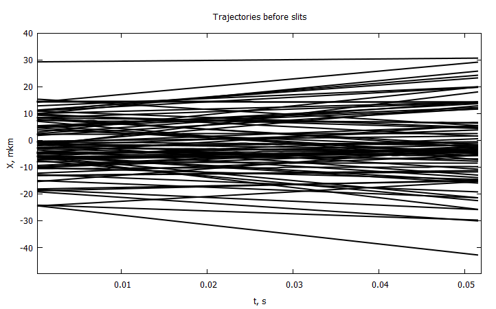

, , , , , . . . , .

Y , , . X . .

" " ,

v_{x} (x, t) = \frac{1}{t - t_{1}} [x + \frac{- 1}{2 (α^{2} + β_{t}^{2})} (β_{t} I m (\frac{C (x, t)}{H (x, t)}) + α Re (\frac{C (x, t)}{H (x, t)}) - β_{t} γ_{x, t})]

$v_{x}(x, t)=\frac{1}{t-t_{1}}\left[x+\frac{-1}{2\left(\alpha^{2}+\beta_{t}^{2}\right)}\left(\beta_{t} I m\left(\frac{C(x, t)}{H(x, t)}\right)+\alpha \operatorname{Re}\left(\frac{C(x, t)}{H(x, t)}\right)-\beta_{t} \gamma_{x, t}\right)\right]$

18+

\begin{aligned} H (x, t) & = \int_{X_{A} - b}^{X_{A} + b} f (x, u, t) d u + \int_{X_{B} - b}^{X_{B} + b} f (x, u, t) d u \\ C (x, t) & = [f (x, u, t)]_{u = X_{A} - b}^{u = X_{A} + b} + [f (x, u, t)]_{u = X_{B} - b}^{u = X_{B} + b} \\ f (x, u, t) & = \exp [(α + i β_{t}) u^{2} + i γ_{x, t} u] \\ α & = - \frac{1}{4 σ_{0}^{2} (1 + {(\frac{ℏ t_{1}}{2 m σ_{0}^{2}})}^{2})} \\ β_{t} & = \frac{m}{2 ℏ} (\frac{1}{t - t_{1}} + \frac{1}{t_{1} (1 + {(\frac{2 m σ_{0}^{2}}{ℏ t_{1}})}^{2})}) \\ γ_{x, t} & = - \frac{m x}{ℏ (t - t_{1})} \end{aligned}

$\begin{aligned} H(x, t) &= \int_{X_{A}-b}^{X_{A}+b} f(x, u, t) d u+\int_{X_{B}-b}^{X_{B}+b} f(x, u, t) d u \\ C(x, t) &= [f(x, u, t)]_{u=X_{A}-b}^{u=X_{A}+b}+[f(x, u, t)]_{u=X_{B}-b}^{u=X_{B}+b} \\ f(x, u, t) &= \exp \left[\left(\alpha+i \beta_{t}\right) u^{2}+i \gamma_{x, t} u\right]\\ \alpha &= -\frac{1}{4 \sigma_{0}^{2}\left(1+\left(\frac{\hbar t_{1}}{2 m \sigma_{0}^{2}}\right)^{2}\right)} \\ \beta_{t} &= \frac{m}{2 \hbar}\left(\frac{1}{t-t_{1}}+\frac{1}{t_{1}\left(1+\left(\frac{2 m \sigma_{0}^{2}}{\hbar t_{1}}\right)^{2}\right)}\right) \\ \gamma_{x, t} &= -\frac{m x}{\hbar\left(t-t_{1}\right)} \end{aligned}$

function Uₓ(t, x)

    γ = -m*x / ( ħ*(t-tf1) )
    β = m/(2ħ) * ( 1/(t-tf1) + 1 / ( tf1*( 1 + (2m*σ₀^2 / (ħ*tf1) )^2 ) ) )
    α = -( 4σ₀^2 * ( 1 + ( ħ*tf1 / (2m*σ₀^2) )^2 ) )^-1

    f(x, u, t) = exp( ( α + im*β )*u^2 + im*γ*u )

    C = f(x, a2, t) - f(x, a1, t) + f(x, b2, t) - f(x, b1, t)
    H = trapez( u-> f(x, u, t) , a1, a2, 400) + trapez( u-> f(x, u, t) , b1, b2, 400)

    return 1/(t-tf1) * ( x - 0.5/(α^2 + β^2) * ( β*imag(C/H) + α*real(C/H) - β*γ ) )
end

init() = bitrand()[1] ? rand()*(b2 - b1) + b1 : rand()*(a2 - a1) + a1
myrng(a, b, N) = collect( range(a, stop = b, length = N ÷ 2) )

n = 1
xx = 0
ξ = 1e-5
while xx < Cron2[end]-Cron2[1]
    n+=1
    xx += (ξ*n)^2 
end
n

steps = [ (ξ*i)^2 for i in 1:n1 ]
Cronadapt = accumulate(+, steps, init = Cron2[1] )

function modelsolver(Np = 10, Nt = 100)

    #xo = [ init() for i = 1:Np ] # 
    xo = vcat( myrng(a2, a1, Np), myrng(b1, b2, Np) ) # 

    xpath = zeros(Nt, Np)
    xpath[1,:] = xo

    for i in 2:Nt, j in 1:Np
        xpath[i,j] = rk4(Uₓ, Cronadapt[i], xpath[i-1,j], steps[i] )
    end

    xpath
end

@time paths = modelsolver(20, n);

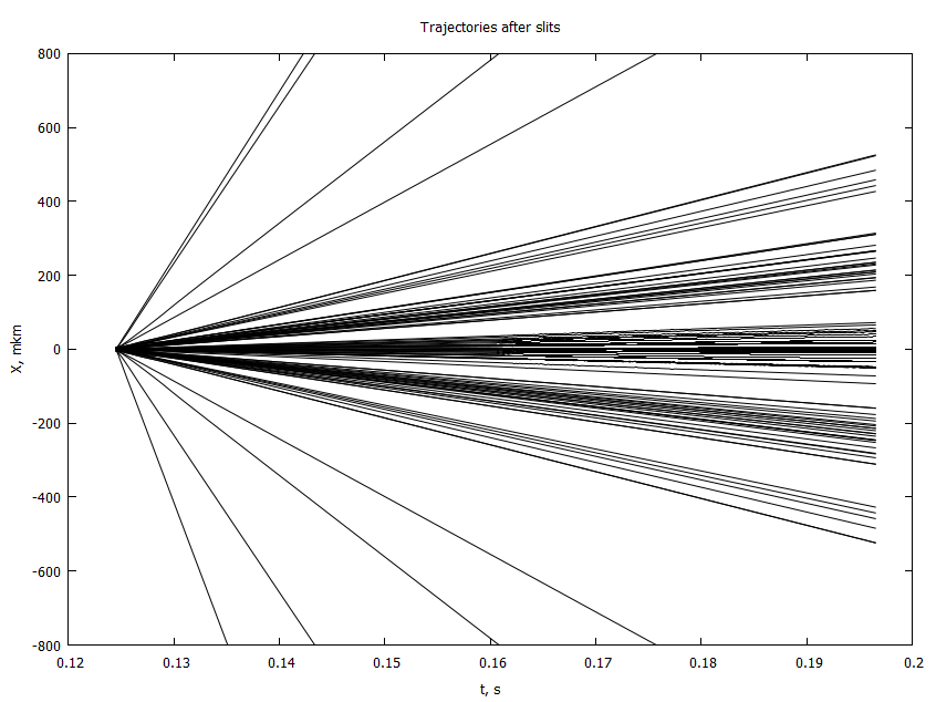
@gp "set title 'Trajectories after the slits'" xlab="t, s" ylab="X, mkm" "set yrange [-800:800]"
for i in 1:size(paths, 2)
    @gp :- Cronadapt 1e6paths[:,i] "with lines notit lw 1 lc rgb 'black'"
end

- 4 , . 2

, : , , .

. , ,

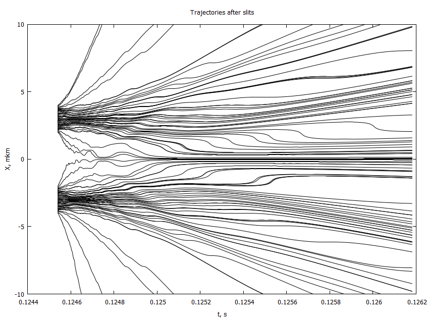
function yas(t, xo, yo, vo)

    cosϕ = xo / sqrt( xo^2 + yo^2 )
    sinϕ = yo / sqrt( xo^2 + yo^2 )
    atnx = -ħ*t / (2m*σ₀^2)
    sinatnx = atnx / sqrt( atnx^2 + 1)
    cosatnx =    1 / sqrt( atnx^2 + 1)
    #cosϕt = cosϕ * cosatnx - sinϕ * sinatnx
    sinϕt = sinϕ*cosatnx + cosϕ*sinatnx

    σ₀t = sqrt( σ₀^2 + ( ħ*t / (2*m*σ₀) )^2 )

    vo*t + sqrt(xo^2 + yo^2) * σ₀t/σ₀ * sinϕt
end

function modelsolver2(Np = 10)

    Nt = length(Cronadapt)
    xo = [ init() for i = 1:Np ]
    #xo = vcat( myrng(a2, a1, Np), myrng(b1, b2, Np) )

    xcoord = copy(xo)
    ycoord = zeros(Np)

    for i in 2:Nt, j in 1:Np
        xcoord[j] = rk4(Uₓ, Cronadapt[i], xcoord[j], steps[i] )
    end

    for (i, x) in enumerate(xo)

        y0 = randn()*yh
        v0 = 0 #randn()*σv*1e-4

        ycoord[i] = yas(Cronadapt[end], x, y0, v0)
    end

    xcoord, ycoord
end

@time X, Y = modelsolver2(100);

@gp "set title 'Impacts on the screen'" xlab="X, mm" ylab="Y, mm"# "set xrange [-1:1]"
@gp :- 1000X 1000Y "with points notit pt 7 ps 0.5 lc rgb 'black'"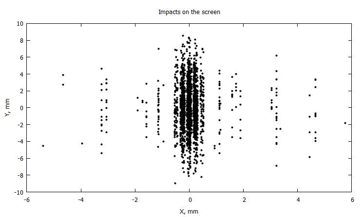

, , . , ,

, , , , , — , .

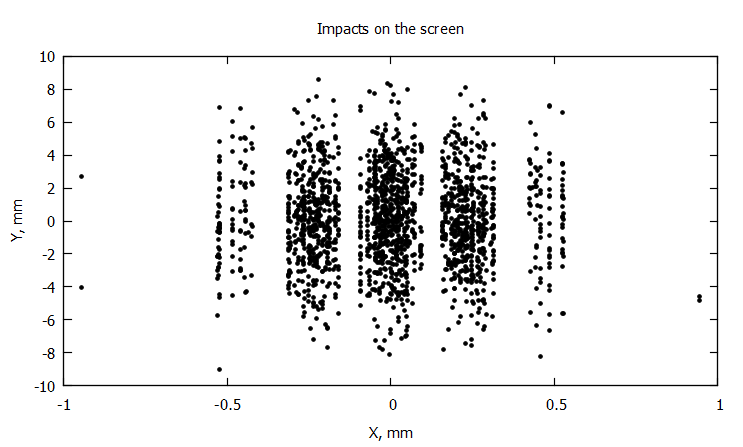
Aplikasi cabul

More articles: