Selamat siang, habraledi dan habragentelmen! Pada artikel ini, kami akan melanjutkan mendalami statistik dengan Python. Jika ada yang melewatkan awal penyelaman, berikut tautan ke bagian pertama . Nah, jika tidak, saya tetap merekomendasikan agar buku terbuka Sarah Boslaf, Statistics for All, tetap dekat. Saya juga merekomendasikan menjalankan notepad untuk bereksperimen dengan kode dan grafik.
Seperti yang dikatakan Andrew Lang, “ Statistik bagi seorang politisi seperti lampu jalan bagi gelandangan mabuk: penyangga daripada penerangan. ” Hal yang sama dapat dikatakan untuk artikel ini untuk pemula. Kecil kemungkinan Anda akan belajar banyak pengetahuan baru di sini, tetapi saya harap artikel ini akan membantu Anda memahami cara menggunakan Python untuk memfasilitasi studi statistik mandiri.
Mengapa menciptakan alokasi baru?
Bayangkan ... jadi, sebelum kita membayangkan apa pun, mari lakukan semua impor yang diperlukan lagi:
import numpy as np
from scipy import stats
import matplotlib.pyplot as plt
import seaborn as sns
from pylab import rcParams
sns.set()
rcParams['figure.figsize'] = 10, 6
%config InlineBackend.figure_format = 'svg'
np.random.seed(42)
, , . , , - , . 1000 100- , . :
gen_pop = np.trunc(stats.norm.rvs(loc=80, scale=5, size=1000))
gen_pop[gen_pop>100]=100
print(f'mean = {gen_pop.mean():.3}')
print(f'std = {gen_pop.std():.3}')
mean = 79.5
std = 4.95
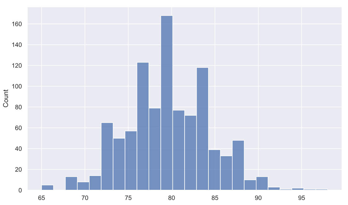
, , . 80 5 . , , , , , - .
, . , - . , - , ? - . , 10 , :
![[89, 99, 93, 84, 79, 61, 82, 81, 87, 82]](https://habrastorage.org/getpro/habr/upload_files/111/47c/b45/11147cb4509f3d49e1c731d87a8b657b.svg)
Z- :

 - ,
- , 
 ,
,  - . :
- . :
sample = np.array([89,99,93,84,79,61,82,81,87,82])
sample.mean()
83.7
Z-:
z = 10**0.5*(sample.mean()-80)/5
z
2.340085468524603
p-value:
1 - (stats.norm.cdf(z) - stats.norm.cdf(-z))
0.019279327322753836
, , : Z- 0 2 , .. 10 , , , 0.02. , 10 , ""  , , 10 "" 83.7 2%. , , , , . .
- 10 , , :
sample.std(ddof=1)
10.055954565441423
ddof std
 , ,
, ,  , . :
, . :

, ,  . -
. - 
 ,
, 
 .
. 
 ? ,
? , 
 -
-  ,
,  .
.  , - .
, - .
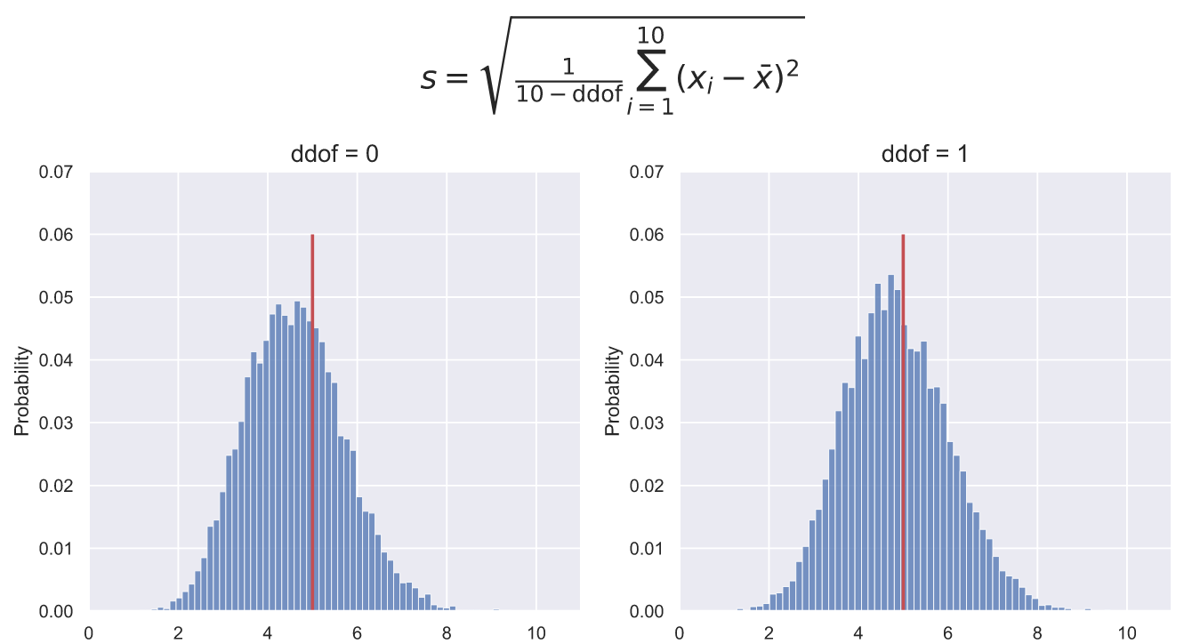
, std() NumPy ddof, 0, std() , , ddof=1. . , 10000 10  , , ddof=0 . ddof=1 , - , ddof=0:
fig, ax = plt.subplots(nrows=1, ncols=2, figsize = (12, 5))
for i in [0, 1]:
deviations = np.std(stats.norm.rvs(80, 5, (10000, 10)), axis=1, ddof=i)
sns.histplot(x=deviations ,stat='probability', ax=ax[i])
ax[i].vlines(5, 0, 0.06, color='r', lw=2)
ax[i].set_title('ddof = ' + str(i), fontsize = 15)
ax[i].set_ylim(0, 0.07)
ax[i].set_xlim(0, 11)
fig.suptitle(r'$s={\sqrt {{\frac {1}{10 - \mathrm{ddof}}}\sum _{i=1}^{10}\left(x_{i}-{\bar {x}}\right)^{2}}}$',
fontsize = 20, y=1.15);
, Z-? , - , . 5000 10 ,  :
:
deviations = np.std(stats.norm.rvs(80, 5, (5000, 10)), axis=1, ddof=1)
sns.histplot(x=deviations ,stat='probability');

, , 10- . . , , 10 2%, , ( ) 10 0. , , : 10- , .
, , , : - , - , . , ""  , Z- p-value 10- :
z = 10**0.5*(sample.mean()-80)/10
p = 1 - (stats.norm.cdf(z) - stats.norm.cdf(-z))
print(f'z = {z:.3}')
print(f'p-value = {p:.4}')
z = 1.17
p-value = 0.242
,  , , , .. ,
  , . 2%, 25%. , -
 .
.
, ? ! , : (, , - )

T-, Z- ,  ,
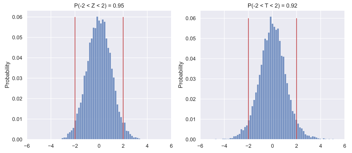
,  . 10000
  , Z- T-, :
fig, ax = plt.subplots(nrows=1, ncols=2, figsize = (12, 5))
N = 10000
samples = stats.norm.rvs(80, 5, (N, 10))
statistics = [lambda x: 10**0.5*(np.mean(x, axis=1) - 80)/5,
lambda x: 10**0.5*(np.mean(x, axis=1) - 80)/np.std(x, axis=1, ddof=1)]
title = 'ZT'
bins = np.linspace(-6, 6, 80, endpoint=True)
for i in range(2):
values = statistics[i](samples)
sns.histplot(x=values ,stat='probability', bins=bins, ax=ax[i])
p = values[(values > -2)&(values < 2)].size/N
ax[i].set_title('P(-2 < {} < 2) = {:.3}'.format(title[i], p))
ax[i].set_xlim(-6, 6)
ax[i].vlines([-2, 2], 0, 0.06, color='r');
- :
import matplotlib.animation as animation
fig, axes = plt.subplots(nrows=1, ncols=2, figsize = (18, 8))
def animate(i):
for ax in axes:
ax.clear()
N = 10000
samples = stats.norm.rvs(80, 5, (N, 10))
statistics = [lambda x: 10**0.5*(np.mean(x, axis=1) - 80)/5,
lambda x: 10**0.5*(np.mean(x, axis=1) - 80)/np.std(x, axis=1, ddof=1)]
title = 'ZT'
bins = np.linspace(-6, 6, 80, endpoint=True)
for j in range(2):
values = statistics[j](samples)
sns.histplot(x=values ,stat='probability', bins=bins, ax=axes[j])
p = values[(values > -2)&(values < 2)].size/N
axes[j].set_title(r'$P(-2\sigma < {} < 2\sigma) = {:.3}$'.format(title[j], p))
axes[j].set_xlim(-6, 6)
axes[j].set_ylim(0, 0.07)
axes[j].vlines([-2, 2], 0, 0.06, color='r')
return axes
dist_animation = animation.FuncAnimation(fig,
animate,
frames=np.arange(7),
interval = 200,
repeat = False)
dist_animation.save('statistics_dist.gif',
writer='imagemagick',
fps=1)
, , . ? -, , . , , ? , , 
![[-2\sigma; 2\sigma]](https://habrastorage.org/getpro/habr/upload_files/f0d/a1c/cfd/f0da1ccfdb352631a44937d502801011.svg) 95.5% . Z- , T- , 92-93% . , , - , :
95.5% . Z- , T- , 92-93% . , , - , :
statistics = [lambda x: 10**0.5*(np.mean(x, axis=1) - 80)/5,
lambda x: 10**0.5*(np.mean(x, axis=1) - 80)/np.std(x, axis=1, ddof=1)]
quantity = 50
N=10000
result = []
for i in range(quantity):
samples = stats.norm.rvs(80, 5, (N, 10))
Z = statistics[0](samples)
p_z = Z[(Z > -2)&((Z < 2))].size/N
T = statistics[1](samples)
p_t = T[(T > -2)&((T < 2))].size/N
result.append([p_z, p_t])
result = np.array(result)
fig, ax = plt.subplots()
line1, line2 = ax.plot(np.arange(quantity), result)
ax.legend([line1, line2],
[r'$P(-2\sigma < {} < 2\sigma)$'.format(i) for i in 'ZT'])
ax.hlines(result.mean(axis=0), 0, 50, color='0.6');
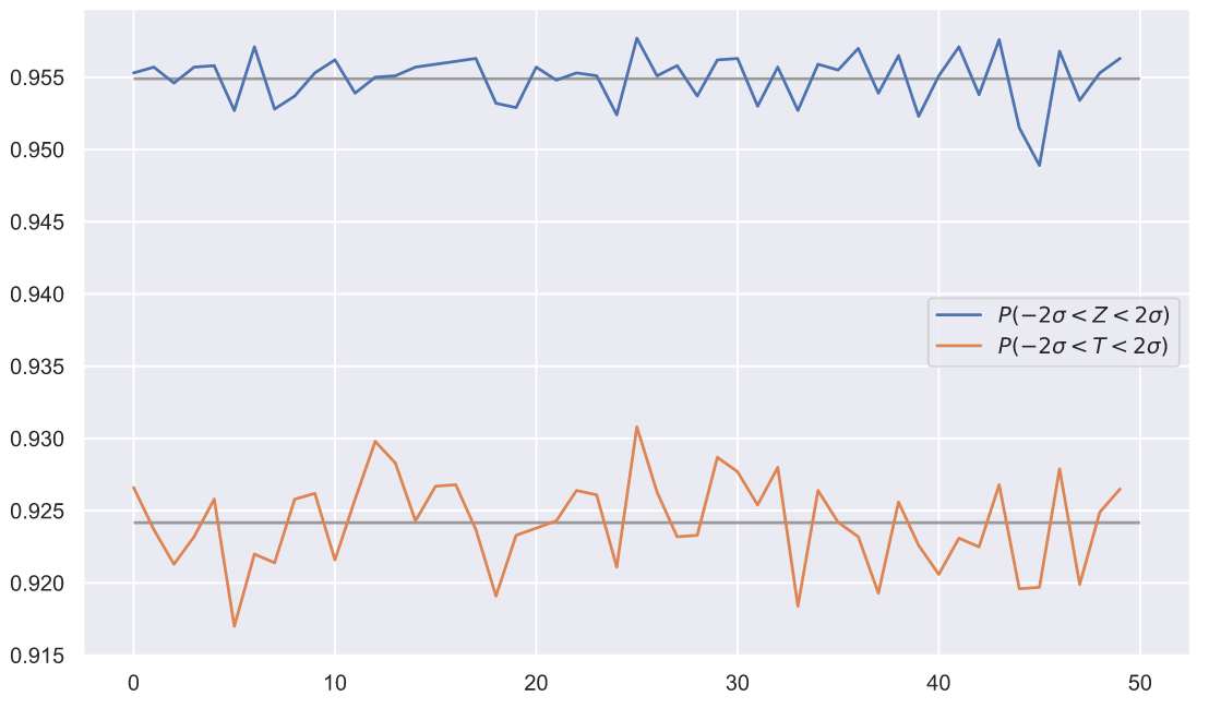
50 . , , , , . ? , ! Z- T- , . , T- ? , - . , , - , , , . , . , - , , 
 .
.
Z-,  ,
,  - . 10000
  10 , :
# ,
# svg png:
#%config InlineBackend.figure_format = 'png'
N = 10000
samples = stats.norm.rvs(80, 5, (N, 10))
means = samples.mean(axis=1)
deviations = samples.std(ddof=1, axis=1)
T = statistics[1](samples)
P = (T > -2)&((T < 2))
fig, ax = plt.subplots()
ax.scatter(means[P], deviations[P], c='b', alpha=0.7,
label=r'$\left | T \right | < 2\sigma$')
ax.scatter(means[~P], deviations[~P], c='r', alpha=0.7,
label=r'$\left | T \right | > 2\sigma$')
mean_x = np.linspace(75, 85, 300)
s = np.abs(10**0.5*(mean_x - 80)/2)
ax.plot(mean_x, s, color='k',
label=r'$\frac{\sqrt{n}(\bar{x}-\mu)}{2}$')
ax.legend(loc = 'upper right', fontsize = 15)
ax.set_title(' \n ',
fontsize=15)
ax.set_xlabel(r' ($\bar{x}$)',
fontsize=15)
ax.set_ylabel(r' ($s$)',
fontsize=15);
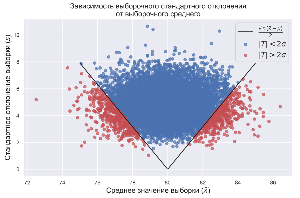
, . , , 
 , .. . , ,
  ,
, 
 . , ( ) , :

,  , .. , , ,
  ,
,  :
:

, ![[-2\sigma; 2\sigma]](https://habrastorage.org/getpro/habr/upload_files/bea/828/453/bea828453e4b32cb920e5d40a188262d.svg) , , 92,5% .
, , 92,5% .
? , . , ( ) 100- . , , ( ). 10- 82- , 2- . , , .  , , ..
  ? Z-:
? Z-:

 p-value:
z = 10**0.5*(82-80)/2
p = 1 - (stats.norm.cdf(z) - stats.norm.cdf(-z))
print(f'p-value = {p:.2}')
p-value = 0.0016
10 82- 2%.  . ,
. ,  , , , .
, , , . (  ) (
) (  ).
).
10 . 82 , , , 9- . ? :
z = 10**0.5*(82-80)/9
p = 1 - (stats.norm.cdf(z) - stats.norm.cdf(-z))
print(f'p-value = {p:.2}')
p-value = 0.48
10 

 . , , - .
, , . :
import matplotlib.animation as animation
fig, ax = plt.subplots(figsize = (15, 9))
def animate(i):
ax.clear()
N = 10000
samples = stats.norm.rvs(80, 5, (N, i))
means = samples.mean(axis=1)
deviations = samples.std(ddof=1, axis=1)
T = i**0.5*(np.mean(samples, axis=1) - 80)/np.std(samples, axis=1, ddof=1)
P = (T > -2)&((T < 2))
prob = T[P].size/N
ax.set_title(r' $s$ $\bar{x}$ $n = $' + r'${}$'.format(i),
fontsize = 20)
ax.scatter(means[P], deviations[P], c='b', alpha=0.7,
label=r'$\left | T \right | < 2\sigma$')
ax.scatter(means[~P], deviations[~P], c='r', alpha=0.7,
label=r'$\left | T \right | > 2\sigma$')
mean_x = np.linspace(75, 85, 300)
s = np.abs(i**0.5*(mean_x - 80)/2)
ax.plot(mean_x, s, color='k',
label=r'$\frac{\sqrt{n}(\bar{x}-\mu)}{2}$')
ax.legend(loc = 'upper right', fontsize = 15)
ax.set_xlim(70, 90)
ax.set_ylim(0, 10)
ax.set_xlabel(r' ($\bar{x}$)',
fontsize='20')
ax.set_ylabel(r' ($s$)',
fontsize='20')
return ax
dist_animation = animation.FuncAnimation(fig,
animate,
frames=np.arange(5, 21),
interval = 200,
repeat = False)
dist_animation.save('sigma_rel.gif',
writer='imagemagick',
fps=3)

, 


 , .
, .  Z-,
Z-,  .
.
! , ? - , , . , , 10- :
![[89,99,93,84,79,61,82,81,87,82]](https://habrastorage.org/getpro/habr/upload_files/e5d/05a/011/e5d05a011425a07da6167192fdea7c18.svg)
 ,
,  , , , , ,
  . Z-, T-, Z- ,
 . , -
. , -  ,
,  - ?
- ?  ?: ,
?: ,  ,
,  ,
, 
 ?
?
, . , - . ,  , , , 10 , 10 . ,
  . , - , .
:  ,
,  ,
, 
 . , ,
. , , 
 :
:
N = 10000
sigma = np.linspace(5, 20, 151)
prob = []
for i in sigma:
p = []
for j in range(10):
samples = stats.norm.rvs(80, i, (N, 10))
means = samples.mean(axis=1)
deviations = samples.std(ddof=1, axis=1)
p_m = means[(means >= 83) & (means <= 84)].size/N
p_d = deviations[(deviations >= 9.5) & (deviations <= 10.5)].size/N
p.append(p_m*p_d)
prob.append(sum(p)/len(p))
prob = np.array(prob)
fig, ax = plt.subplots()
ax.plot(sigma, prob)
ax.set_xlabel(r' ($\sigma$)',
fontsize=20)
ax.set_ylabel('',
fontsize=20);
,  . , ,
. , ,  ,
,  . - , , , , . .
T-?
, - - . 1% , - . , , . , - -. ?
- ! , - , "" t-. , , , . , , 1943 , 50% . , - .
, "" . , ( !) , "" , :

t-, . , , "", , , , , - . " ", "t-" , .
:

" " .  , ..
, ..  ,
,  , .. , . - , :

, :
import matplotlib.animation as animation
fig, ax = plt.subplots(figsize = (15, 9))
def animate(i):
ax.clear()
N = 15000
x = np.linspace(-5, 5, 100)
ax.plot(x, stats.norm.pdf(x, 0, 1), color='r')
samples = stats.norm.rvs(0, 1, (N, i))
t = samples[:, 0]/np.sqrt(np.mean(samples[:, 1:]**2, axis=1))
t = t[(t>-5)&(t<5)]
sns.histplot(x=t, bins=np.linspace(-5, 5, 100), stat='density', ax=ax)
ax.set_title(r' $t(n)$ n = ' + str(i), fontsize = 20)
ax.set_xlim(-5, 5)
ax.set_ylim(0, 0.5)
return ax
dist_animation = animation.FuncAnimation(fig,
animate,
frames=np.arange(2, 21),
interval = 200,
repeat = False)
dist_animation.save('t_rel_of_df.gif',
writer='imagemagick',
fps=3)
,  , , ,
, , ,  . , , :

SciPy:
import matplotlib.animation as animation
fig, ax = plt.subplots(figsize = (15, 9))
def animate(i):
ax.clear()
N = 15000
x = np.linspace(-5, 5, 100)
ax.plot(x, stats.norm.pdf(x, 0, 1), color='r')
ax.plot(x, stats.t.pdf(x, df=i))
ax.set_title(r' $t(n)$ n = ' + str(i), fontsize = 20)
ax.set_xlim(-5, 5)
ax.set_ylim(0, 0.45)
return ax
dist_animation = animation.FuncAnimation(fig,
animate,
frames=np.arange(2, 21),
interval = 200,
repeat = False)
dist_animation.save('t_pdf_rel_of_df.gif',
writer='imagemagick',
fps=3)

,  ( df ) . - , ,
  , .
, .
t-
t- SciPy :
sample = np.array([89,99,93,84,79,61,82,81,87,82])
stats.ttest_1samp(sample, 80)
Ttest_1sampResult(statistic=1.163532240174695, pvalue=0.2745321678073461)
:
T = 9**0.5*(sample.mean() -80)/sample.std()
T
1.163532240174695
,  ,
,  ,
,  . , 1 , , , . :
T = 10**0.5*(sample.mean() -80)/sample.std(ddof=1)
T
1.1635322401746953
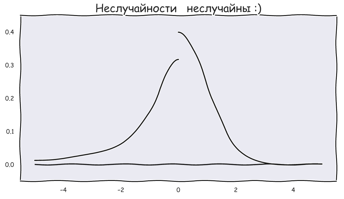
, t- , p-value? , - , p-value Z-, t-:
t = stats.t(df=9)
fig, ax = plt.subplots()
x = np.linspace(t.ppf(0.001), t.ppf(0.999), 300)
ax.plot(x, t.pdf(x))
ax.hlines(0, x.min(), x.max(), lw=1, color='k')
ax.vlines([-T, T], 0, 0.4, color='g', lw=2)
x_le_T, x_ge_T = x[x<-T], x[x>T]
ax.fill_between(x_le_T, t.pdf(x_le_T), np.zeros(len(x_le_T)), alpha=0.3, color='b')
ax.fill_between(x_ge_T, t.pdf(x_ge_T), np.zeros(len(x_ge_T)), alpha=0.3, color='b')
p = 1 - (t.cdf(T) - t.cdf(-T))
ax.set_title(r'$P(\left | T \right | \geqslant {:.3}) = {:.3}$'.format(T, p));

, p-value 27%, .. , - ,  , p-value , 5 . , , - ,
  , 0.95:

SciPy, interval loc () scale () :
sample_loc = sample.mean()
sample_scale = sample.std(ddof=1)/10**0.5
ci = stats.t.interval(0.95, df=9, loc=sample_loc, scale=sample_scale)
ci
(76.50640345566619, 90.89359654433382)
,  , ,
, , 
![[76,5; 90,9]](https://habrastorage.org/getpro/habr/upload_files/271/4c8/21d/2714c821d6a7a520116d1a2df7c3059c.svg) . , ,
. , ,  , .
, .
, , , ( ). , , t- , t- , t- .
Tentu saja, saya ingin memasukkan beberapa gif di akhir, tetapi saya ingin mengakhiri dengan kalimat dari Herbert Spencer: " Tujuan terbesar dari pendidikan bukanlah pengetahuan, tetapi tindakan ", jadi luncurkan anakonda Anda dan ambil tindakan ! Ini terutama berlaku untuk orang otodidak seperti saya.
Saya menekan F5 dan menantikan komentar Anda!