Tanggal dan waktu bukanlah hal yang mudah:
- bulan berisi jumlah hari yang berbeda;
- tahun adalah tahun kabisat dan bukan;
- ada zona waktu yang berbeda;
- jam, menit, hari menggunakan sistem angka yang berbeda;
- dan masih banyak lagi nuansa lainnya.
Berikut ini adalah ringkasan dari beberapa poin yang jarang disorot dalam dokumentasi, serta trik yang memungkinkan Anda menulis kode dengan cepat dan terkontrol.
Rangkuman yang sangat singkat untuk pembaca ponsel cerdas: pada data dalam jumlah besar, kami hanya menggunakan POSIXct
sebagian kecil detik. Ini akan bagus, tentu saja, dengan cepat.
Ini adalah kelanjutan dari serangkaian publikasi sebelumnya .
Standar untuk Menentukan Tanggal dan Waktu
ISO 8601 Elemen data dan format pertukaran - Pertukaran informasi - Representasi tanggal dan waktu adalah standar internasional yang mencakup pertukaran data terkait tanggal dan waktu.
Metode R Dasar untuk Bekerja dengan Waktu
tanggal
Sys.Date()
print("-----")
x <- as.Date("2019-01-29") # UTC
print(x)
tz(x)
str(x)
dput(x)
print("-----")
dput(as.Date("1970-01-01")) # ! origin
## [1] "2021-04-29" ## [1] "-----" ## [1] "2019-01-29" ## [1] "UTC" ## Date[1:1], format: "2019-01-29" ## structure(17925, class = "Date") ## [1] "-----" ## structure(0, class = "Date")
Format tanggal non-standar selama inisialisasi harus ditentukan secara khusus
as.Date("04/20/2011", format = "%m/%d/%Y")
## [1] "2011-04-20"
Waktu
Ada dua tipe waktu dasar yang digunakan di R: POSIXct
dan POSIXlt
.
Tampilan luar POSIXct
dan POSIXlt
terlihat serupa. Dan yang internal?
z <- Sys.time()
glue(" ",
"POSIXct - {z}",
"POSIXlt - {as.POSIXlt(z)}", "---", .sep = "\n")
glue(" ",
"POSIXct - {capture.output(dput(z))}",
"POSIXlt - {paste0(capture.output(dput(as.POSIXlt(z))), collapse = '')}",
"---", .sep = "\n")
# /
glue(": {year(z)} \n: {minute(z)}\n: {second(z)}\n---")
## ## POSIXct - 2021-04-29 15:18:04 ## POSIXlt - 2021-04-29 15:18:04 ## --- ## ## POSIXct - structure(1619698684.50764, class = c("POSIXct", "POSIXt")) ## POSIXlt - structure(list(sec = 4.50764489173889, min = 18L, hour = 15L, mday = 29L, mon = 3L, year = 121L, wday = 4L, yday = 118L, isdst = 0L, zone = "MSK", gmtoff = 10800L), class = c("POSIXlt", "POSIXt"), tzone = c("", "MSK", "MSD")) ## --- ## : 2021 ## : 18 ## : 4 ## ---
Segera kami menyimpulkan bahwa untuk pekerjaan serius dengan data (lebih dari 10 baris seiring waktu), kami POSIXlt
melupakannya sebagai mimpi buruk. Ini adalah struktur yang kompleks dengan overhead yang tidak masuk akal.
POSIXct
unixtimestamp, () ( 0 01.01.1970). .
— online unixtimestamp:
- Epoch Unix Time Stamp Converter
- Epoch & Unix Timestamp Conversion Tools
- currentDate / Time in Millisecondsmillis
z <- 1548802400
as.POSIXct(z, origin = "1970-01-01") # local
as.POSIXct(z, origin = "1970-01-01", tz = "UTC") # in UTC
## [1] "2019-01-30 01:53:20 MSK" ## [1] "2019-01-29 22:53:20 UTC"
. . :
- ISO, (ISO 8601-2019);
- - ;
- .
POSIXct
, - . :
x <- ymd_hms("2014-09-24 15:23:10")
x
x + 0.5
x + 0.5 + 0.6
options(digits.secs=5)
x + 0.45756
options(digits.secs=0)
x
## [1] "2014-09-24 15:23:10 UTC" ## [1] "2014-09-24 15:23:10 UTC" ## [1] "2014-09-24 15:23:11 UTC" ## [1] "2014-09-24 15:23:10.45756 UTC" ## [1] "2014-09-24 15:23:10 UTC"
, .
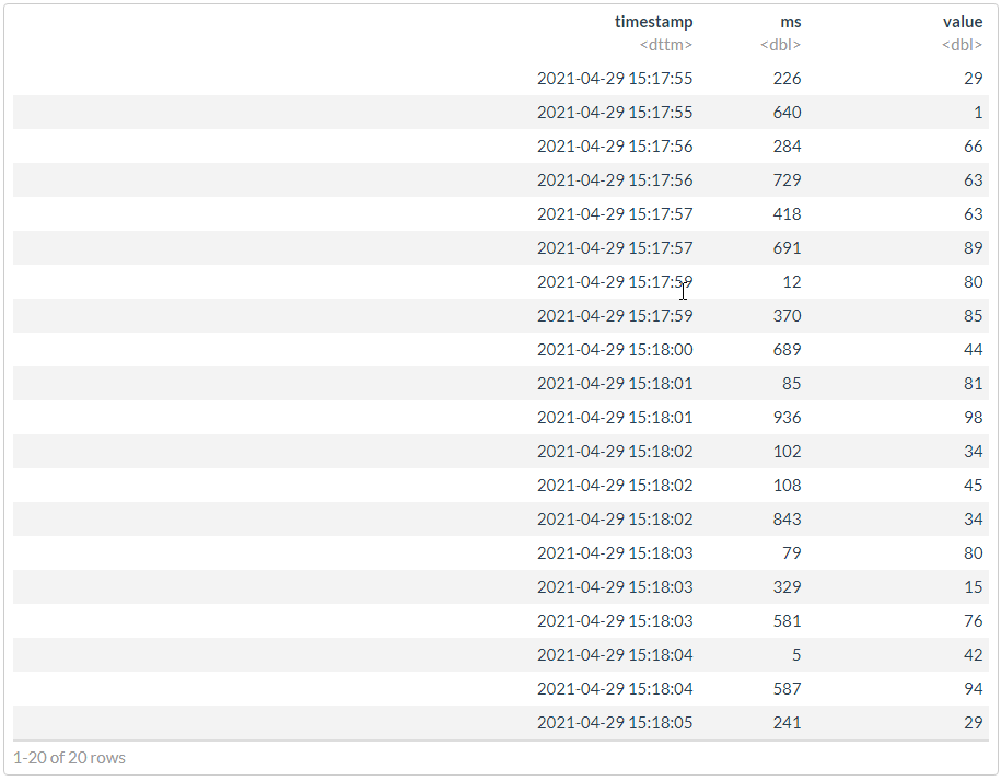
options(digits.secs=5)
# generate data
df <- data.frame(
timestamp = as_datetime(
round(runif(20, min = now() - seconds(10), max = now()), 0),
tz ="Europe/Moscow")) %>%
mutate(ms = round(runif(n(), 0, 999), 0)) %>%
mutate(value = round(runif(n(), 0, 100), 0))
dput(df)
# " "
df %>%
arrange(timestamp, ms)
options(digits.secs=0)
## structure(list(timestamp = structure(c(1619698677, 1619698680, ## 1619698676, 1619698682, 1619698675, 1619698682, 1619698679, 1619698679, ## 1619698684, 1619698683, 1619698684, 1619698677, 1619698682, 1619698683, ## 1619698675, 1619698676, 1619698685, 1619698681, 1619698683, 1619698681 ## ), class = c("POSIXct", "POSIXt"), tzone = "Europe/Moscow"), ## ms = c(418, 689, 729, 108, 226, 843, 12, 370, 5, 581, 587, ## 691, 102, 79, 640, 284, 241, 85, 329, 936), value = c(63, ## 44, 63, 45, 29, 34, 80, 85, 42, 76, 94, 89, 34, 80, 1, 66, ## 29, 81, 15, 98)), class = "data.frame", row.names = c(NA, ## -20L))
# ""
# [magrittr aliases](https://magrittr.tidyverse.org/reference/aliases.html)
df2 <- df %>%
mutate(timestamp = timestamp + ms/1000) %>%
# mutate_at("timestamp", ~`+`(. + ms/1000)) %>%
select(-ms) %>%
df2 %>% arrange(timestamp)

#
dt <- as.data.table(df2)
bench::mark(
naive = dplyr::arrange(df, timestamp, ms),
smart = dplyr::arrange(df2, timestamp),
dt = dt[order(timestamp)],
check = FALSE,
relative = TRUE,
min_iterations = 1000
)
## # A tibble: 3 x 6 ## expression min median `itr/sec` mem_alloc `gc/sec` ## <bch:expr> <dbl> <dbl> <dbl> <dbl> <dbl> ## 1 naive 11.9 11.8 1 1.06 1 ## 2 smart 11.1 11.0 1.06 1 1.06 ## 3 dt 1 1 11.6 494. 1.22
.
data <- c("05102019210003657", "05102019210003757", "05102019210003857")
dmy_hms(stri_c(stri_sub(data, to = 14L), ".", stri_sub(data, from = 15L)), tz = "Europe/Moscow")
#
data2 <- data %>%
sample(10^6, replace = TRUE)
bench::mark(
stri_sub = stri_c(stri_sub(data2, to = 14L), ".", stri_sub(data2, from = 15L)),
stri_replace = stri_replace_first_regex(data2, pattern = "(^.{14})(.*)", replacement = "$1.$2"),
re2_replace = re2_replace(data2, pattern = "(^.{14})(.*)", replacement = "\\1.\\2", parallel = TRUE)
)
## [1] "2019-10-05 21:00:03 MSK" "2019-10-05 21:00:03 MSK" ## [3] "2019-10-05 21:00:03 MSK" ## # A tibble: 3 x 6 ## expression min median `itr/sec` mem_alloc `gc/sec` ## <bch:expr> <bch:tm> <bch:tm> <dbl> <bch:byt> <dbl> ## 1 stri_sub 214ms 222ms 4.10 22.89MB 5.47 ## 2 stri_replace 653ms 653ms 1.53 7.63MB 0 ## 3 re2_replace 409ms 413ms 2.42 15.29MB 1.21
lubridate
x <- ymd(20101215)
print(x)
class(x)
## [1] "2010-12-15" ## [1] "Date"
lubridate
ymd(20101215) == mdy("12/15/10")
## [1] TRUE
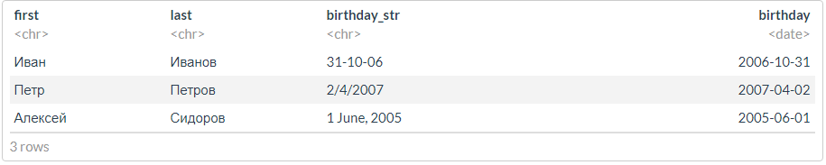
df <- tibble(first = c("", "", ""),
last = c("", "", ""),
birthday_str = c("31-10-06", "2/4/2007", "1 June, 2005")) %>%
mutate(birthday = dmy(birthday_str))
df
, ?
# lubridate
options(lubridate.verbose = TRUE)
# : ..
df <- tibble(time_str = c("08.05.19 12:04:56", "09.05.19 12:05", "12.05.19 23"))
lubridate::dmy_hms(df$time_str, tz = "Europe/Moscow")
print("---------------------")
lubridate::dmy(df$time_str, tz = "Europe/Moscow")
## [1] "2019-05-08 12:04:56 MSK" NA ## [3] NA ## [1] "---------------------" ## [1] NA NA NA
# lubridate
options(lubridate.verbose = TRUE)
lubridate::dmy_hms(df$time_str, truncated = 3, tz = "Europe/Moscow")
## [1] "2019-05-08 12:04:56 MSK" "2019-05-09 12:05:00 MSK" ## [3] "2019-05-12 23:00:00 MSK"
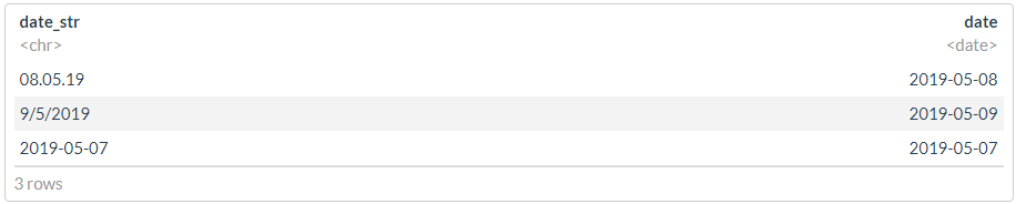
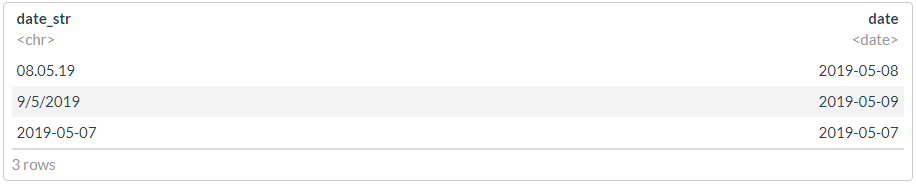
# lubridate
options(lubridate.verbose = TRUE)
# : ..
df <- tibble(date_str = c("08.05.19", "9/5/2019", "2019-05-07"))
#
glimpse(dmy(df$date_str))
print("---------------------")
#
glimpse(ymd(df$date_str))
print("---------------------")
## Date[1:3], format: "2019-05-08" "2019-05-09" NA ## [1] "---------------------" ## Date[1:3], format: "2008-05-19" NA "2019-05-07" ## [1] "---------------------"
? , , , - .
df %>% mutate(date = dplyr::coalesce(dmy(date_str), ymd(date_str)))
df1 <- df
df1$date <- dmy(df1$date_str)
idx <- is.na(df1$date)
print("---------------------")
idx
df1$date[idx] <- ymd(df1$date_str[idx])
print("---------------------")
df1
## [1] "---------------------" ## [1] FALSE FALSE TRUE ## [1] "---------------------"
"" :
POSIXct
options(lubridate.verbose = FALSE)
date1 <- ymd_hms("2011-09-23-03-45-23")
date2 <- ymd_hms("2011-10-03-21-02-19")
# ?
as.numeric(date2) - as.numeric(date1) # ,
(date2 - date1) %>% dput()
difftime(date2, date1)
difftime(date2, date1, unit="mins")
difftime(date2, date1, unit="secs")
## [1] 926216 ## structure(10.7200925925926, class = "difftime", units = "days") ## Time difference of 10.72009 days ## Time difference of 15436.93 mins ## Time difference of 926216 secs
date1 <- ymd_hms("2019-01-30 00:00:00")
date1
date1 - days(1)
date1 + days(1)
date1 + days(2)
## [1] "2019-01-30 UTC" ## [1] "2019-01-29 UTC" ## [1] "2019-01-31 UTC" ## [1] "2019-02-01 UTC"
—
date1 - months(1)
date1 + months(1) # !!!
## [1] "2018-12-30 UTC" ## [1] NA
. , .
date1 %m-% months(1)
date1 %m+% months(1)
date1 %m+% months(1) %m-% months(1)
## [1] "2018-12-30 UTC" ## [1] "2019-02-28 UTC" ## [1] "2019-01-28 UTC"
date1 <- ymd_hms("2019-01-30 01:00:00")
date1 %T>% print() %>% dput()
with_tz(date1, tzone = "Europe/Moscow") %T>% print() %>% dput()
force_tz(date1, tzone = "Europe/Moscow") %T>% print() %>% dput()
## [1] "2019-01-30 01:00:00 UTC" ## structure(1548810000, class = c("POSIXct", "POSIXt"), tzone = "UTC") ## [1] "2019-01-30 04:00:00 MSK" ## structure(1548810000, class = c("POSIXct", "POSIXt"), tzone = "Europe/Moscow") ## [1] "2019-01-30 01:00:00 MSK" ## structure(1548799200, class = c("POSIXct", "POSIXt"), tzone = "Europe/Moscow")
, , ? , hms
. .
hms_str <- "03:22:14"
as_hms(hms_str)
dput(as_hms(hms_str))
print("-------")
x <- as_hms(hms_str) * 15
x
str(x)
# seconds_to_period(period_to_seconds(x))
seconds_to_period(x) %T>% dput() %>% print()
## 03:22:14 ## structure(12134, units = "secs", class = c("hms", "difftime")) ## [1] "-------" ## Time difference of 182010 secs ## 'difftime' num 182010 ## - attr(*, "units")= chr "secs" ## new("Period", .Data = 30, year = 0, month = 0, day = 2, hour = 2, ## minute = 33) ## [1] "2d 2H 33M 30S"
— . .
( Clickhouse) , , unixtimestamp UTC. , .
:
- . timestamp, , , , , .
- ( ). , , , .
- unixtimestamp UTC , . (!).
- , timestamp. ,
X-1
X+1
, .
, 0.
.
(, ) . , :
- , ;
- ;
- ;
- ( );
- ;
-
double
; - ;
- .
-- ClickHouse
SELECT DISTINCT
store, pos,
timestamp, ms,
concat(toString(store), '-', toString(pos)) AS pos_uid,
toFloat64(timestamp) + (ms / 1000) AS timestamp
flog.info(paste("SQL query:", sql_req))
tic(" CH")
raw_df <- dbGetQuery(conn, stri_encode(sql_req, to = "UTF-8")) %>%
mutate_if(is.character, `Encoding<-`, "UTF-8") %>%
as_tibble() %>%
mutate_at(vars(timestamp), anytime::anytime, tz = "Europe/Moscow") %>%
mutate_at("event", as.factor)
flog.info(capture.output(toc()))
DBI::dbDisconnect(conn)
data.frame
#
df -> as_tibble(_df) %>%
map(pryr::object_size) %>%
unlist() %>%
enframe() %>%
arrange(desc(value)) %>%
mutate_at("value", fs::as_fs_bytes) %>%
mutate(ratio = formattable::percent(value / sum(value), 2)) %>%
add_row(name = "TOTAL", value = sum(.$value))
,
- Epoch & Unix Timestamp Conversion Tools
- currentdate/time in millisecondsmillis
- Functions for working with dates and times
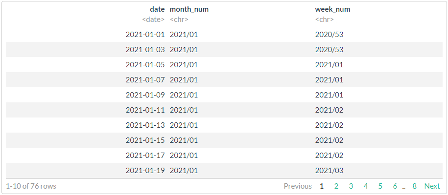
, , , . .
df <- seq.Date(from = as.Date("2021-01-01"),
to = as.Date("2021-05-31"),
by = "2 days") %>%
# sample(20, replace = FALSE) %>%
tibble(date = .)
# //
# 1
df %>%
mutate(month_num = stri_c(lubridate::year(date),
sprintf("%02d", lubridate::month(date)),
sep = "/"),
week_num = stri_c(lubridate::isoyear(date),
sprintf("%02d", lubridate::isoweek(date)),
sep = "/")
)
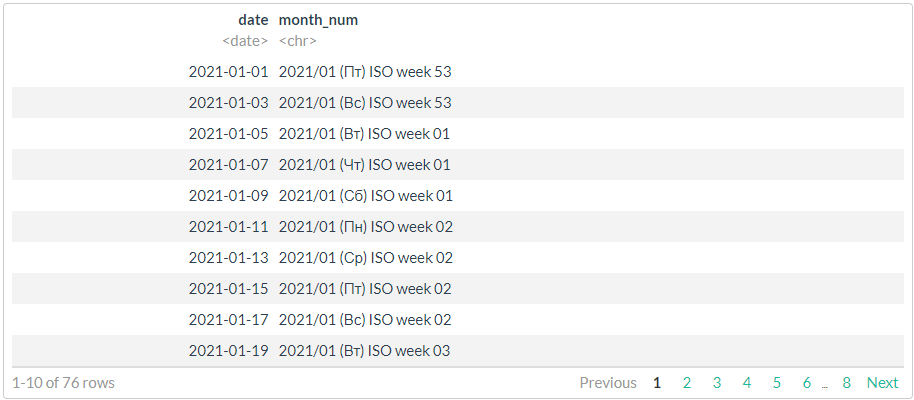
# //
# 2,
# , !!!
df %>%
mutate(month_num = format(date, "%Y/%m (%a) ISO week %V"))
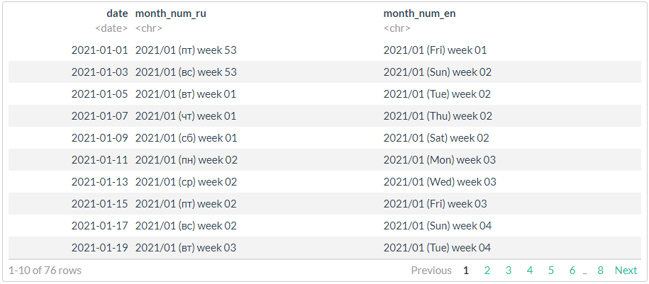
# //
# 3,
# strptime (ISO 8601) ICU
# https://man7.org/linux/man-pages/man3/strptime.3.html
stri_datetime_fstr("%Y/%m (%a) week %V")
# ggthemes::tableau_color_pal("Tableau 20")(20) %>% scales::show_col()
# , !!!
df %>%
mutate(
month_num_ru = stri_datetime_format(
date, "yyyy'/'MM' ('ccc') week 'ww", locale = "ru", tz = "UTC"),
month_num_en = stri_datetime_format(
date, "yyyy'/'MM' ('ccc') week 'ww", locale = "en", tz = "UTC"))
. .
stri_datetime_format(today(), "LLLL", locale="ru@calendar=Persian")
stri_datetime_format(today(), "LLLL", locale="ru@calendar=Indian")
stri_datetime_format(today(), "LLLL", locale="ru@calendar=Hebrew")
stri_datetime_format(today(), "LLLL", locale="ru@calendar=Islamic")
stri_datetime_format(today(), "LLLL", locale="ru@calendar=Coptic")
stri_datetime_format(today(), "LLLL", locale="ru@calendar=Ethiopic")
stri_datetime_format(today(), "dd MMMM yyyy", locale="ru")
stri_datetime_format(today(), "LLLL d, yyyy", locale="ru")
## [1] "" ## [1] "" ## [1] "" ## [1] "" ## [1] "" ## [1] "" ## [1] "29 2021" ## [1] " 29, 2021"
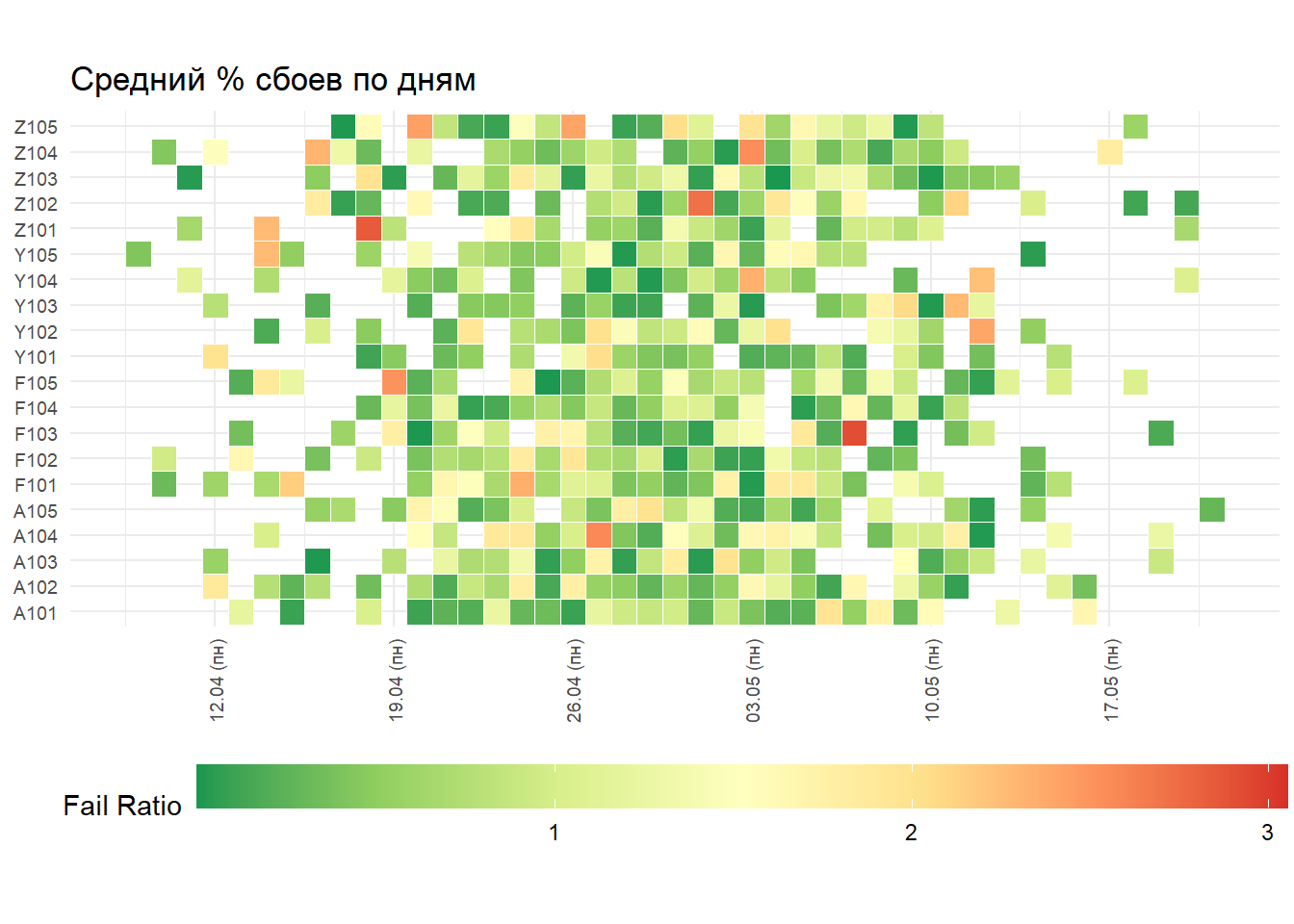
.
#
map_tbl <- tibble(
date = as_date(Sys.time() + rnorm(10^3, mean = 0, sd = 60 * 60 * 24 * 7))) %>%
mutate(store = stri_c(sample(c("A", "F", "Y", "Z"), n(), replace = TRUE),
sample(101:105, n(), replace = TRUE))) %>%
mutate(store_fct = as.factor(store)) %>%
mutate(fail_ratio = abs(rnorm(n(), mean = 0.3, sd = 1)))
my_date_format <- function (format = "dd MMMM yyyy", tz = "Europe/Moscow")
{
scales:::force_all(format, tz)
# stri_datetime_fstr("%d.%m%n%A")
# stri_datetime_fstr("%d.%m (%a)")
function(x) stri_datetime_format(x, format, locale = "ru", tz = tz)
}
# ,
gp <- map_tbl %>%
ggplot(aes(x = date, y = store_fct, fill = fail_ratio)) +
geom_tile(color = "white", size = 0.1) +
# scale_fill_distiller(palette = "RdYlGn", name = "Fail Ratio", label = comma) +
# scale_fill_distiller(palette = "RdYlGn", name = "Fail Ratio", guide = guide_legend(keywidth = unit(4, "cm"))) +
scale_fill_distiller(palette = "RdYlGn", name = "Fail Ratio") +
scale_x_date(breaks = scales::date_breaks("1 week"), labels = my_date_format("dd'.'MM' ('ccc')'")) +
coord_equal() +
labs(x = NULL, y = NULL, title = " % ") +
theme_minimal() +
theme(plot.title = element_text(hjust = 0)) +
theme(axis.ticks = element_blank()) +
theme(axis.text = element_text(size = 7)) +
theme(axis.text.x = element_text(angle = 90, vjust = 0.5)) +
theme(legend.position = "bottom") +
theme(legend.key.width = unit(3, "cm"))
gp
base_df <- tibble(
start = Sys.time() + rnorm(10^3, mean = 0, sd = 60 * 24 * 3)) %>%
mutate(finish = start + rnorm(n(), mean = 100, sd = 60)) %>%
mutate(user_id = sample(as.character(1000:1100), n(), replace = TRUE)) %>%
arrange(user_id, start)
dt <- as.data.table(base_df, key = c("user_id", "start")) %>%
.[, c("start", "finish") := lapply(.SD, as.numeric),
.SDcols = c("start", "finish")]
df <- group_by(base_df, user_id)
bench::mark(
dplyr_v1 = df %>% transmute(delta_t = as.numeric(difftime(finish, start, units = "secs"))) %>% ungroup(),
dplyr_v2 = ungroup(df) %>% transmute(delta_t = as.numeric(difftime(finish, start, units = "secs"))),
dplyr_v3 = dt %>% transmute(delta_t = finish - start),
dt_v1 = dt[, .(delta_t = finish - start), by = user_id],
dt_v2 = dt[, .(delta_t = finish - start)],
check = FALSE # all_equal
)
## # A tibble: 5 x 6 ## expression min median `itr/sec` mem_alloc `gc/sec` ## <bch:expr> <bch:tm> <bch:tm> <dbl> <bch:byt> <dbl> ## 1 dplyr_v1 4.3ms 4.86ms 200. 103.1KB 11.4 ## 2 dplyr_v2 2.17ms 2.46ms 380. 17.9KB 6.24 ## 3 dplyr_v3 1.67ms 1.77ms 527. 29.8KB 8.51 ## 4 dt_v1 410.4us 438.7us 2139. 90.8KB 8.35 ## 5 dt_v2 304.4us 335.3us 2785. 264.6KB 8.38
: //. , , ?
Kode sampel. Jangan lupa bahwa sejumlah fungsi bekerja dengan mempertimbangkan lokal mesin tempat kode dijalankan. Dan jika bulan Anda dicetak dalam bahasa Rusia, maka ini tidak menjamin (jika Anda tidak menggunakan metode) perilaku serupa di komputer lain atau OS lain.
# https://stackoverflow.com/questions/16347731/how-to-change-the-locale-of-r
# https://jangorecki.gitlab.io/data.cube/library/stringi/html/stringi-locale.html
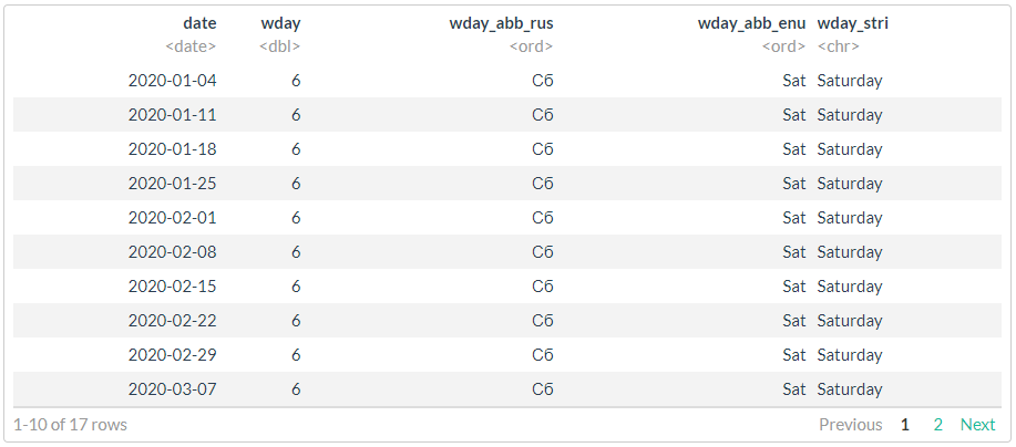
df <- as.Date("2020-01-01") %>%
seq.Date(to = . + months(4), by = "1 day") %>%
tibble(date = .) %>%
mutate(wday = lubridate::wday(date, week_start = 1),
wday_abb_rus = lubridate::wday(date, label = TRUE, week_start = 1),
wday_abb_enu = lubridate::wday(date, label = TRUE, week_start = 1, locale = "English"),
wday_stri = stringi::stri_datetime_format(date, "EEEE", locale = "en"))
#
filter(df, wday == 6)
PS Sebagian besar tes hanya sebagai contoh. Anda dapat menjalankannya di mesin Anda, angkanya akan sangat berbeda, tetapi sifat ketergantungan dan rasionya harus kurang lebih sama.
Posting sebelumnya - "R vs Python dalam loop produktif" .