Di kota yang bagus dekat Moskow, ada perlintasan kereta api yang buruk. Selama jam sibuk tidak hanya naik, tetapi juga persimpangan dan jalan tetangga. Mengemudi sekali lagi, saya bertanya-tanya - berapa kapasitasnya dan dapatkah ada yang diubah?

Untuk jawabannya, kita akan mempelajari sedikit tentang peraturan dan teori arus lalu lintas, menganalisis data GPS dan akselerometer menggunakan Python dan membandingkan perhitungan teoritis dengan data eksperimen.
Kandungan
1.
, 10 /. .
Jupyter Notebook GitHub'.

:
import pandas as pd
import numpy as np
import glob

#!pip install utm
import utm

from sklearn.decomposition import PCA
from scipy import interpolate

import matplotlib.pyplot as plt
import seaborn as sns
sns.set(rc={'figure.figsize':(12, 8)})
import plotly.express as px

#  Mapbox    Plotly
mapbox_token = open('mapbox_token', 'r').read()
2.
.
— 1 .
— .
— , .
— , - .
:
.
« » . , 2005 . , .

218.2.020-2012 " ".
, :
— , , , .
, :
, , .
2 :
- ;
- .
:
- :
,
,
– () , – , – , , — . ( ): .
- :
,
— ( ), — () ( ). 218.2.020-2012 —
#
diagram1 = pd.read_csv('  .csv', sep=';', header=None, names=['P', 'V'], decimal=',')
diagram1_func = interpolate.interp1d(diagram1['P'], diagram1['V'], kind='cubic')
diagram1_xnew = np.arange(diagram1['P'].min(), diagram1['P'].max())

#
diagram2 = pd.read_csv(' .csv', sep=';', header=None, names=['P', 'Q'], decimal=',')
diagram2_func = interpolate.interp1d(diagram2['P'], diagram2['Q'], kind='cubic')
diagram2_xnew = np.arange(diagram2['P'].min(), diagram2['P'].max())
def density_Tanaka(V):
#
V = V * 1000 / 60 / 60 # / /
L = 5.7 #
c1 = 0.504 #
c2 = 0.0285 #**2/
return 1000 / (L + c1 * V + c2 * V**2) # ./
def density_Grindshilds(V):
#
pmax = 85 # ./
vmax = 60 # /
return pmax * (1 - V / vmax) # ./#
V = np.arange(1, 80) # /
V1 = np.arange(1, 61) # /
fig, (ax1, ax2) = plt.subplots(1, 2, figsize=(16, 8))
ax1.plot(density_Tanaka(V), V, label=" ")
ax1.plot(density_Grindshilds(V1), V1, label=" ")
ax1.plot(diagram1_xnew, diagram1_func(diagram1_xnew), label=". ")
ax1.set_xlabel(r' $\rho$, /')
ax1.set_ylabel(r' $V$, /')
ax1.legend()
ax2.plot(density_Tanaka(V), density_Tanaka(V) * V, label=" ")
ax2.plot(density_Grindshilds(V1), density_Grindshilds(V1) * V1, label=" ")
ax2.plot(diagram2_xnew, diagram2_func(diagram2_xnew), label=". ")
ax2.set_xlabel(r' $\rho$, /')
ax2.set_ylabel(r' $Q$, /')
ax2.legend()
plt.show()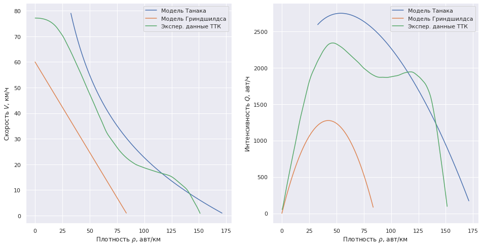
. .
3.
3.1
, . Enter, :
%%writefile "key-logger.py"
import pandas as pd
import time
import datetime

class _GetchUnix:
    # from https://code.activestate.com/recipes/134892/
    def __init__(self):
        import tty, sys

    def __call__(self):
        import sys, tty, termios
        fd = sys.stdin.fileno()
        old_settings = termios.tcgetattr(fd)
        try:
            tty.setraw(sys.stdin.fileno())
            ch = sys.stdin.read(1)
        finally:
            termios.tcsetattr(fd, termios.TCSADRAIN, old_settings)
        return ch

def logging():
    path = 'logs/keylog/'
    filename = f"{time.strftime('%Y-%m-%d %H-%M-%S')}.csv"
    path_to_file = path + filename
    db = []
    getch = _GetchUnix()
    print('...')
    while True:
        key = getch()
        if key == 'c':
            break
        else:
            db.append((datetime.datetime.now(), key))
    df = pd.DataFrame(db, columns=['time', 'click'])
    print(df)
    df.to_csv(path_to_file, index=False)
    print(f"\nSaved to {filename}")

if __name__ == "__main__":
    logging()
20 . 2 , . . 100%:
files = glob.glob('logs/keylog/*.csv')
keylogger_data = []
print(f'  - {len(files)} .')
for filename in files:
    df = pd.read_csv(filename, parse_dates=['time'])
    keylogger_data.append(df)
keylogger_data = pd.concat(keylogger_data, ignore_index=True)
keylogger_data.head()| time | click | |
|---|---|---|
| 0 | 2020-09-29 16:24:02.691189 | d |
| 1 | 2020-09-29 16:24:05.186670 | a |
| 2 | 2020-09-29 16:24:07.157702 | d |
| 3 | 2020-09-29 16:24:11.506961 | a |
| 4 | 2020-09-29 16:24:14.206266 | a |
"a" — , 'd' — .
:
keylogger_data['time'] = keylogger_data['time'].astype('datetime64[m]')
keylogger_per_min = keylogger_data.groupby(['click', 'time'], as_index=False).size().reset_index().rename(columns={0:'size'})
keylogger_per_min.head()| index | click | time | size | |
|---|---|---|---|---|
| 0 | 0 | a | 2020-09-29 16:24:00 | 12 |
| 1 | 1 | a | 2020-09-29 16:25:00 | 13 |
| 2 | 2 | a | 2020-09-29 16:26:00 | 9 |
| 3 | 3 | a | 2020-09-29 16:27:00 | 18 |
| 4 | 4 | a | 2020-09-29 16:28:00 | 14 |
sns.catplot(x='click', y='size', kind="box", data=keylogger_per_min);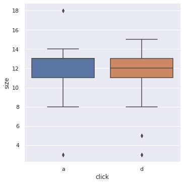
print(f"  : {keylogger_per_min['size'].mean():.1f} ./ \
 {keylogger_per_min['size'].mean() * 60:.1f} ./")
: 11.7 ./ 700.0 ./
.
— 700 ./ 10 / ( 50 / ) — .
plt.plot(V1, density_Grindshilds(V1)*V1, label=" ")
plt.xlabel(r' $V$, /')
plt.ylabel(r' $Q$, /')
plt.show()
3.2
Android GPSLogger csv . ( ) GPS — Physics Toolbox Suite.
50 . — .
, — .
GPSLogger
GPSLogger , :
- time — ;
- lat lon — , ;
- speed — , ;
- direction — , .
files = glob.glob('logs/gps/*.csv')
gpslogger_data = []
print(f'    GPS - {len(files)} .')
for filename in files:
    df = pd.read_csv(filename, parse_dates=['time'], index_col='time')
    if df.iloc[10, 1] < df.iloc[-1, 1]:
        df['direction'] = 0 #
    else:
        df['direction'] = 1 #
    gpslogger_data.append(df)
gpslogger_data = pd.concat(gpslogger_data)
gpslogger_data.head()

gps_1 = gpslogger_data[['lat', 'lon', 'speed', 'direction']]
GPS — 37 .
Physics Toolbox Suite:
files = glob.glob('logs/gps_accel/*.csv')
print(f'     - {len(files)} .')
pts_data = []

for filename in files:
    df = pd.read_csv(filename, sep=';',decimal=',')
    df['time'] = filename[-22:-12] + '-' + df['time']
    if df.iloc[10, 5] < df.iloc[-1, 5]:
        df['direction'] = 0 #
    else:
        df['direction'] = 1 #
    pts_data.append(df)
pts_data = pd.concat(pts_data)
pts_data.head()
— 14 .
| time | ax | ay | az | Latitude | Longitude | Speed (m/s) | Unnamed: 7 | direction | |
|---|---|---|---|---|---|---|---|---|---|
| 0 | 2020-09-04-14:11:18:029 | 0.0 | 0.0 | 0.0 | 0.000000 | 0.00000 | 0.0 | NaN | 1 |
| 1 | 2020-09-04-14:11:18:030 | 0.0 | 0.0 | 0.0 | 56.372343 | 37.53044 | 0.0 | NaN | 1 |
| 2 | 2020-09-04-14:11:18:030 | 0.0 | 0.0 | 0.0 | 56.372343 | 37.53044 | 0.0 | NaN | 1 |
| 3 | 2020-09-04-14:11:18:094 | 0.0 | 0.0 | 0.0 | 56.372343 | 37.53044 | 0.0 | NaN | 1 |
| 4 | 2020-09-04-14:11:18:094 | 0.0 | 0.0 | 0.0 | 56.372343 | 37.53044 | 0.0 | NaN | 1 |
, — :
pts_data = pts_data.query('Latitude != 0.')Physics Toolbox Suite 400 , GPS 1 , :
pts_data['time'] = pd.to_datetime(pts_data['time'], format='%Y-%m-%d-%H:%M:%S:%f')
pts_data = pts_data.rename(columns={'Latitude':'lat', 'Longitude':'lon', 'Speed (m/s)':'speed'})
:
accel_data = pts_data[['time', 'lat', 'lon', 'ax', 'ay', 'az', 'direction']].copy()
accel_data = accel_data.set_index('time')
accel_data['direction'] = accel_data['direction'].map({1.: ' ', 0.: ' '})
accel_data.head()| lat | lon | ax | ay | az | direction | |
|---|---|---|---|---|---|---|
| time | ||||||
| 2020-09-04 14:11:18.030 | 56.372343 | 37.53044 | 0.0 | 0.0 | 0.0 | |
| 2020-09-04 14:11:18.030 | 56.372343 | 37.53044 | 0.0 | 0.0 | 0.0 | |
| 2020-09-04 14:11:18.094 | 56.372343 | 37.53044 | 0.0 | 0.0 | 0.0 | |
| 2020-09-04 14:11:18.094 | 56.372343 | 37.53044 | 0.0 | 0.0 | 0.0 | |
| 2020-09-04 14:11:18.095 | 56.372343 | 37.53044 | 0.0 | 0.0 | -0.0 |
GPS:
gps_2 = pts_data[['time', 'lat', 'lon', 'speed', 'direction']].copy()
gps_2 = gps_2.set_index('time')
gps_2 = gps_2.resample('S').mean()
gps_2 = gps_2.dropna(how='all')
gps_2.head()| lat | lon | speed | direction | |
|---|---|---|---|---|
| time | ||||
| 2020-08-10 00:45:02 | 56.338342 | 37.522946 | 0.0 | 1.0 |
| 2020-08-10 00:45:03 | 56.338342 | 37.522946 | 0.0 | 1.0 |
| 2020-08-10 00:45:04 | 56.338342 | 37.522946 | 0.0 | 1.0 |
| 2020-08-10 00:45:05 | 56.338342 | 37.522946 | 0.0 | 1.0 |
| 2020-08-10 00:45:06 | 56.338342 | 37.522946 | 0.0 | 1.0 |
GPS :
gps_data = gps_1.append(gps_2, ignore_index=True)
gps_data['direction'] = gps_data['direction'].map({1.: ' ', 0.: ' '})
gps_data.head()| lat | lon | speed | direction | |
|---|---|---|---|---|
| 0 | 56.167241 | 37.504026 | 19.82 | |
| 1 | 56.167051 | 37.503804 | 19.36 | |
| 2 | 56.166884 | 37.503667 | 19.62 | |
| 3 | 56.166718 | 37.503554 | 19.35 | |
| 4 | 56.166570 | 37.503427 | 19.12 |
3.2.1
Plotly:
fig = px.scatter_mapbox(gps_data, lat="lat", lon="lon", color='direction', zoom=17, height=600)
fig.update_layout(mapbox_accesstoken=mapbox_token, mapbox_style='streets')
fig.show()
3.2.2
:
- GPS, WGS 84 .
- .
Web Mercator, — , , .
, . — , — (UTM).
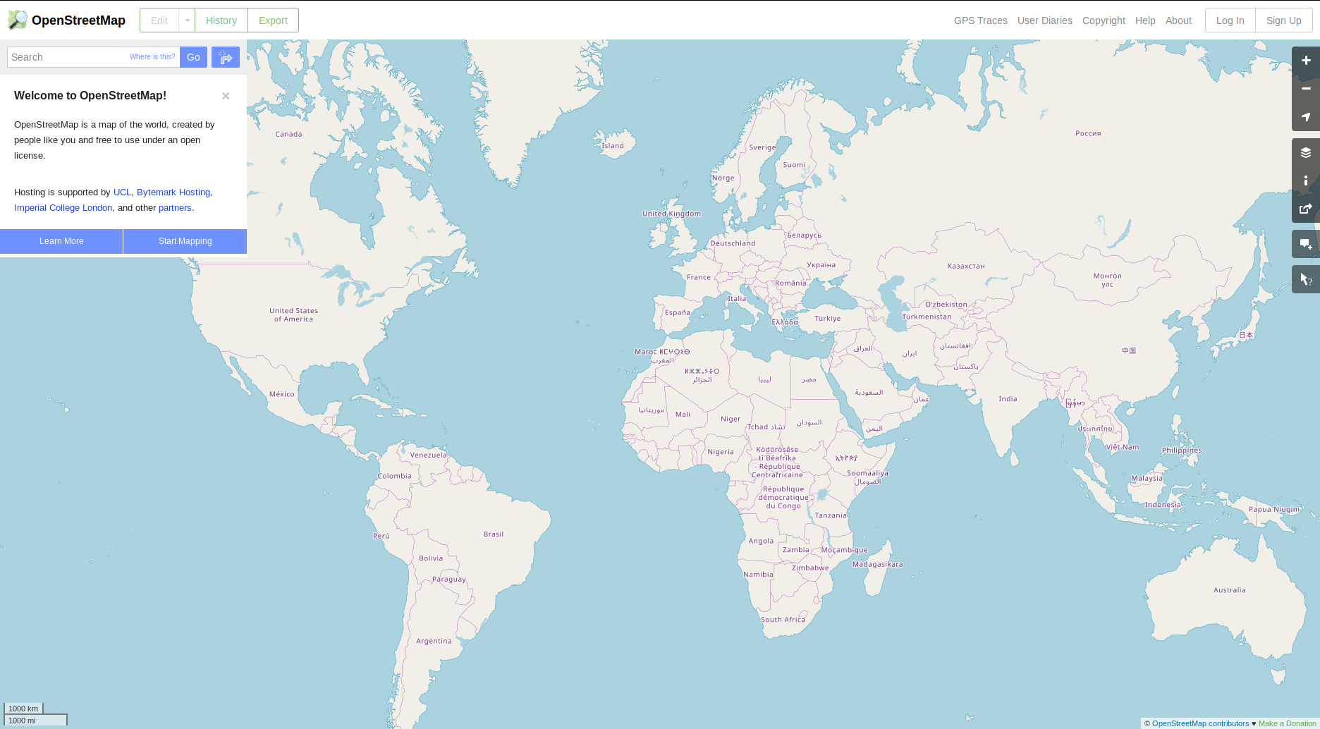
Web-Mercator
UTM
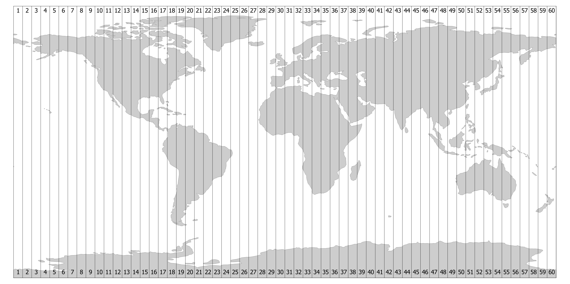
UTM Python https://github.com/Turbo87/utm, .
gps_data['xs'] = gps_data[['lat', 'lon']].apply(lambda x: utm.from_latlon(x[0], x[1])[0], axis=1)
gps_data['ys'] = gps_data[['lat', 'lon']].apply(lambda x: utm.from_latlon(x[0], x[1])[1], axis=1)
gps_data['speed_kmh'] = gps_data.speed / 1000 * 60 * 60
50 :
#
lat0 = 56.35205
lon0 = 37.51792
xc, yc, _, _ = utm.from_latlon(lat0, lon0)

r = 50
gps_data = gps_data.query(f'{xc - r} < xs & xs < {xc + r}')\
                   .query(f'{yc - r} < ys & ys < {yc + r}')
fig = px.scatter_mapbox(gps_data, lat="lat", lon="lon", color='direction', zoom=17, height=600)
fig.update_layout(mapbox_accesstoken=mapbox_token, mapbox_style='streets')
fig.show()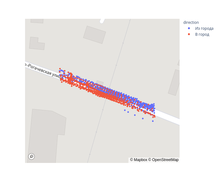
. 2d 1d, (PCA).
2 — scikit-learn. Sklearn:
pca = PCA(n_components=1).fit(gps_data[['xs', 'ys']])
gps_data['xs_transform'] = pca.transform(gps_data[['xs', 'ys']])sns.relplot(x='xs_transform', y='speed_kmh', data=gps_data, aspect=2.5, hue='direction');
. — [-5, 25]. .
accel_data['xs'] = accel_data[['lat', 'lon']].apply(lambda x: utm.from_latlon(x[0], x[1])[0], axis=1)
accel_data['ys'] = accel_data[['lat', 'lon']].apply(lambda x: utm.from_latlon(x[0], x[1])[1], axis=1)
accel_data = accel_data.query(f'{xc - r} < xs & xs < {xc + r}')\
                       .query(f'{yc - r} < ys & ys < {yc + r}')
accel_data['xs_transform'] = pca.transform(accel_data[['xs', 'ys']])
Android :

( Y). :
sns.relplot(x='xs_transform', y='ax', data=accel_data, aspect=2.5, hue='direction');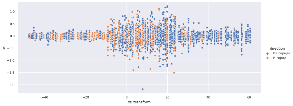
sns.relplot(x='xs_transform', y='ay', data=accel_data, aspect=2.5, hue='direction');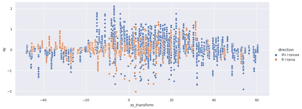
sns.relplot(x='xs_transform', y='az', data=accel_data, aspect=2.5, hue='direction');
Z:
sns.relplot(x='xs_transform', y='az', data=accel_data.query('-20 < xs_transform < 40'), aspect=2.5, hue='direction');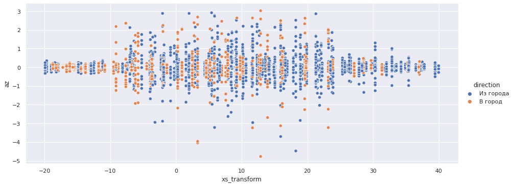
X Z — [-10, 25] 7.5.
cross = gps_data.query('-10 < xs_transform < 25')fig = px.scatter_mapbox(cross, lat="lat", lon="lon", color='direction', zoom=19, height=600)
fig.update_layout(mapbox_accesstoken=mapbox_token, mapbox_style='streets')
fig.show()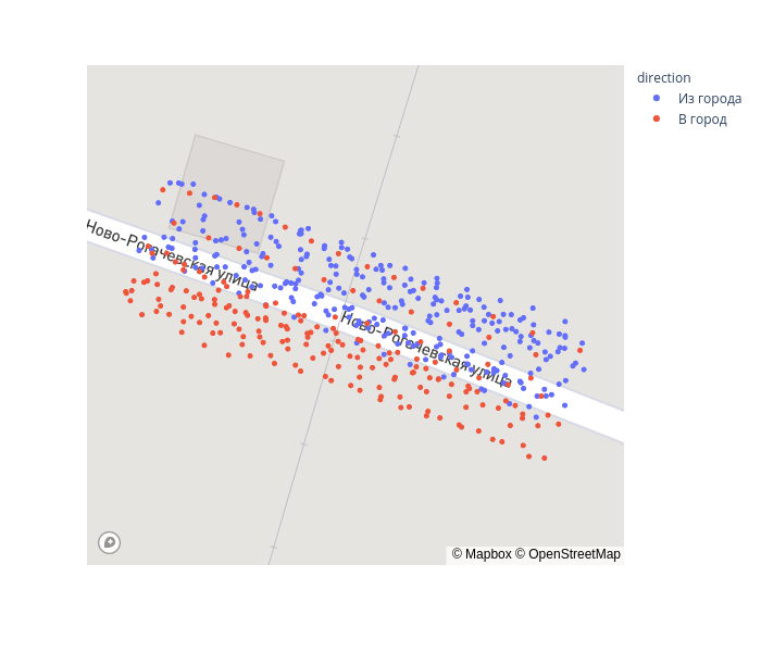
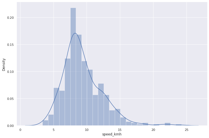
:
mean_v = cross.speed_kmh.mean()
print(f"    - {mean_v:.2} /")
sns.distplot(cross.speed_kmh);
— 9.4 /
:
base = 1
gps_data['xs_transform_round'] = gps_data['xs_transform'].apply(lambda x: base * round(x / base))
accel_data['xs_transform_round'] = accel_data['xs_transform'].apply(lambda x: base * round(x / base))sns.relplot(x='xs_transform_round', y='speed_kmh', data=gps_data, kind="line", aspect=2.5);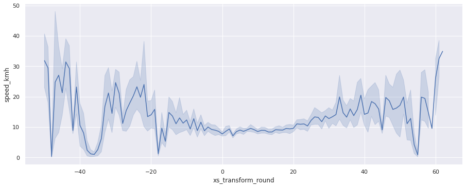
sns.relplot(x='xs_transform_round', y='az', data=accel_data, kind="line", aspect=2.5);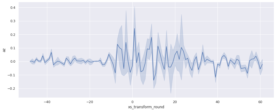
3.3
:
gps_data['flow_Tanaka'] = density_Tanaka(gps_data.speed_kmh) * gps_data.speed_kmh
gps_data['flow_Grindshilds'] = density_Grindshilds(gps_data.speed_kmh) * gps_data.speed_kmhsns.relplot(x='xs_transform_round', y='flow_Grindshilds', data=gps_data, aspect=2.5, kind='line', hue='direction');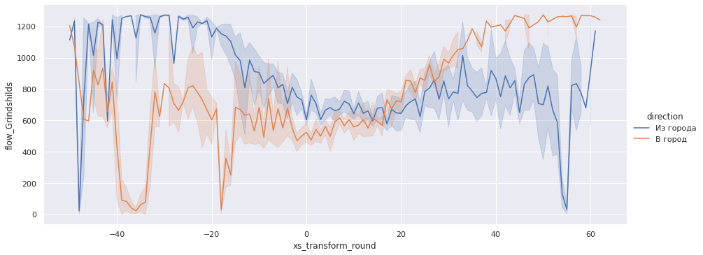
cross = gps_data.query('-10 < xs_transform < 25')mean_flow_Tanaka = cross.flow_Tanaka.mean()
print(f" - {mean_flow_Tanaka:.1f} / \
{mean_flow_Tanaka / 60:.1f} /")— 1275.5 / 21.3 /
mean_flow_Grindshilds = cross.flow_Grindshilds.mean()
print(f"      - {mean_flow_Grindshilds:.1f} / \
 {mean_flow_Grindshilds / 60:.1f} /")
— 660.0 / 11.0 /
, 700 ./.
plt.plot(V1, density_Grindshilds(V1)*V1, label=" ")
plt.xlabel(r' $V$, /')
plt.ylabel(r' $Q$, /')
plt.show()
, - 30 / — .
, :
4.
Berdasarkan analisis kami, dapat dikatakan bahwa perlintasan sebidang berada dalam kondisi yang tidak memuaskan dan kecepatan aliran sekitar 10 km / jam, yang apabila jalan penuh akan menyebabkan masalah lalu lintas dan kemacetan lalu lintas.
Throughput penyeberangan dapat ditingkatkan secara signifikan dengan membawa penyeberangan pada kondisi yang memuaskan.